Scientific Computing in Finance
- MATH-GA 2048, Spring 2020
- Courant Institute of Mathematical Sciences, New York University
Objectives of this class
- Teach fundamental principles of scientific computing
- Teach the most common numerical techniques in quantitative Finance
- Develop intuitions and essential skills using real world examples
- Help students to start a career in quantitative Finance
We expect you
- Know basic calculus and linear algebra
- Know basic stochastic calculus and derivative pricing theories
- Have some prior programming experience
- Are willing to learn through hard work
Main fields of quantitative finance
- Derivative pricing and hedging
- Risk management, regulatory capital and stress testing
- Portfolio management
- Quantitative strategy/Algo trading
- Behavior models
We will cover many topics in the first three fields.
Main topics in this class
A rough schedule of the class:
| Week | Main Topics | Practical Problems | Instructor |
|---|---|---|---|
| 1 | Introduction and Error Analysis | Error and floating point numbers | H. Cheng |
| 2-3 | Linear Algebra | Portfolio optimization, PCA, least square | H. Cheng |
| 4-5 | Rootfinding and interpolation | Curve building | H. Cheng |
| 6 | Derivatives and integration | Hedging, Risk Transformation | H. Cheng |
| 7-8 | Monte Carlo simulation | Exotic pricing | H. Cheng |
| 9-10 | Optimization | Model calibration | W. Lou |
| 11-13 | ODE/PDE | Pricing | W. Lou |
Text book
D Bindel and J Goodman, 2009
- Principles of scientific computing online book
References
L Anderson and V. Piterbarg, 2010
- Interest rate modeling, volume I: Foundations and Vanilla Models
- Interest rate modeling, volume II: Vanilla Models
P. Glasserman 2010
- Monte Carlo method in Financial Engineering
Lecture notes and homework
Available online at: http://yadongli.github.io/nyumath2048
Grading
- Homework 50%, can be done by groups of two students
- Final 50%
- Extra credits
- extra credit homework problems
- for pointing out errors in slides/homework
Software Development Practices
Roberto Waltman: In the one and only true way. The object-oriented version of "Spaghetti code" is, of course, "Lasagna code".
Modern hardware
- Processor speed/throughput continues to grow at an impressive rate
- Moore's law has ruled for a long time
- recent trends: multi-core, GPU, TPU
- Memory capacity continues to grow, but memory speed only grows at a (relatively) slow rate
Memory hierarchy
| Storage | Bandwidth | Latency | Capacity |
|---|---|---|---|
| L-1 Cache | 98GB/s | 4 cycles | 32K/core |
| L-2 Cache | 50GB/s | 10 cycles | 256K/core |
| L-3 Cache | 30GB/s | 40 - 75 cycles | 8MB shared |
| RAM | 15GB/s | 60-100 ns | ~TB |
| SDD | up to 4GB/s | ~0.1ms | $\infty$ |
| Network | up to 12GB/s | much longer | $\infty$ |
On high performance computing
- Understand if the problem is computation or bandwidth bound
- Most problems in practice are bandwidth bound
- Computation bound problems:
- caching
- vectorization/parallelization/GPU
- optimize your "computational kernel"
- Bandwidth bound problems:
- optimize cache and memory access
- require highly specialized skills and low level programming (like in C/C++/Fortran)
- Premature optimization for speed is the root of all evil
- Simplicity, generality and scalability of the code are often sacrificed
- Execution speed is often not the most critical factor in most circumstances
Before optimizing for speed
- Correctness
- "those who would give up correctness for a little temporary performance deserve neither correctness nor performance"
- "the greatest performance improvement of all is when system goes from not-working to working"
- Modifiability
- "modification is undesirable but modifiability is paramount"
- modular design, learn from hardware designers
- Simplicity
- no obvious defects is not the same as obviously no defects
- Other desirable features:
- Scalability, robustness, Easy support and maintenance etc.
In practice, what often trumps everything else is:
Time to market !!
- First mover has significant advantage: Facebook, Google etc.
Conventional advice for programming
- Choose good names for your variables and functions
- Write comments and documents
- Write good tests
- Keep coding style consistent
These are good advice, but quite superficial.
- all of them have been compromised, even in very successful projects
- they are usually not the critical differentiator between successes and failures
Best advice for the real world:
by Paul Phillips "We're doing it all wrong":
(quoting George Orwell's 1984)
War is peace
- Fight your war at the boundary so that you can have peace within
- Challenge your clients to reduce the scope of your deliverable
- Define a minimal set of interactions to the outside world
Ignorance is strength
- Design dumb modules that only do one thing
- Keep it simple and stupid
- Separation of concerns, modular
Freedom is slavery
- Must be disciplined in testing, code review, releases etc.
- Limit the interface of your module (or external commitments)
- Freedom $\rightarrow$ possibilities $\rightarrow$ complexity $\rightarrow$ unmodifiable code $\rightarrow$ slavery
Less is more
Sun Tzu (孙子): "the supreme art of quant modeling is to solve problems without coding"
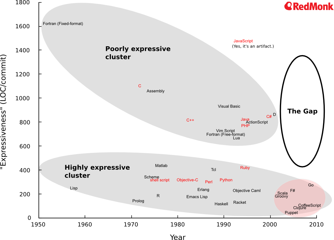
Choose the right programming tools
- Programming paradigm: procedural, OOP, functional
- Expressivity: fewer lines of code for the same functionality
- Ecosystem: library, tools, community, industry support
There is no single right answer
- Different job calls for different tools
- But most of the time, the choice is already made (by someone else)
Eric Raymond, "How to Become a Hacker":
"Lisp is worth learning for the profound enlightenment experience you will have when you finally get it; that experience will make you a better programmer for the rest of your days, even if you never actually use Lisp itself a lot."
- Clojure is a modern implementation of Lisp
- Julia is a very promising new language, heavily influenced by Lisp
We use Python for this class
Python
- a powerful dynamic and strongly typed scripting language
- extremely popular in scientific computing
- strong momentum in quantitative finance
- highly productive, low learning curve
Python ecosystem
- numpy/scipy: high quality matrix and numerical library
- matplotlib: powerful visualization library
- Jupyter notebook: highly productive interactive working environment
- Pandas: powerful data and time series analysis package
- Machine learning frameworks: Tensorflow, PyTorch, Scikit-learn etc.
Python resources
- Anaconda: a popular Python distribution with essential packages, best choice
- Enthought Canopy: a commercial Python distribution, free for students
- Google and Youtube
Python version:
- Python 3.6.x only ( version 3.7.x is not supported currently) : python is not backward compatible, do not use Python 2
- With the latest Jupyter notebook, numpy/pandas/scipy etc.
- either 32bit or 64bit version works
Python setup instructions:
- available at: http://yadongli.github.io/nyumath2048
Errors and floating point computation
James Gosling: "95% of the folks out there are completely clueless about floating-point"
Absolute and relative error
If the true value $a$ is approximated by $\hat{a}$:
- Absolute error: $\hat{a} - a$
- Relative error: $\frac{\hat{a} - a}{a}$
Both measure are useful in practice.
- Beware of small $|a|$ when comparing relative errors
Sources of error
Imprecision in the theory or model itself
- George Box: "essentially, all models are wrong, but some are useful"
Truncation Error in numerical algorithm: introduced when exact mathematical formulae are represented by approximations.
- Convergence error
- Monte Carlo simulation
- Numerical integration
- Truncation and discretization
- Termination of iterations
Roundoff Errors: occur because computers have a limited ability to represent numbers
- Floating point number
- Rounding
We cover the last category in this lecture.
IEEE 754 in a nutshell
First published in 1985, the IEEE 754 standard includes:
- Floating point number representations
- 16bit, 32bit, 64bit etc
- special representation for NaN, Inf etc
- Rounding rules
- Basic operations
- arithmetic: add, multiplication, sqrt etc
- conversion: btw formats, to/from string etc
- Exception handling
- invalid operation, divide by zero, overflow, underflow, inexact
- the operation returns a value (could be NaN, Inf or 0), and set an error flag
Rounding under IEEE754
Default rule: round to the nearest, ties to even digit
- Example, round to 4 significant digit(bit):
- decimal: $3.12450 \rightarrow 3.1240$, $435150 \rightarrow 435200$
- binary: $10.11100 \rightarrow 11.00$, $1100100 \rightarrow 1100000 $
- Addition and multiplication are commutative with rounding, but not associative
- Intermediate calculations could be done at higher precision to minimize numerical error, if supported by the hardware
- Intel CPU's FPU can use 80bit representation for intermediate calculations, even if input/outputs are in 64/32 bit floats
- Early version of Java (before v1.2) enforces intermediate calculation to be in 32/64bits for float/double for binary compatibility - a poor choice
Importance of IEEE 754
IEEE 754 is a tremendously successful standard:
- Allows users to consistently reason about floating point computation
- before IEEE 754, floating point number calculation behaves differently across different platforms
- IEEE 754 made compromise for practicality
- many of them do not make strict mathematical sense
- but they are necessary evils for the greater goods
- Establishes a clear interface between hardware designers and software developers
- Its main designer, William Kahan won the Turing award in 1989
The IEEE 754 standard is widely adopted in modern hardware and software,
- The vast majority of general purpose CPUs are IEEE 754 compliant
- Software is more complicated
- Compiled language like C++ depends on the hardware's implementation.
- Some software implemented their own special behaviours, e.g., the Java strictfp flag
IEEE 754 floating point number format
- IEEE floating point number standard
$$\underbrace{*}_{\text{sign bit}}\;\underbrace{********}_{\text{exponent}}\overbrace{\;1.\;}^{\text{implicit}}\;\underbrace{***********************}_{\text{fraction}} $$
$$(-1)^{\text{sign}}(\text{1 + fraction})2^{\text{exponent} - p}$$
- 32 bit vs. 64 bit format
| Format | Sign | Fraction | Exponent | $p$ | (Exponent-p) range |
|---|---|---|---|---|---|
| IEEE 754 - 32 bit | 1 | 23 | 8 | 127 | -126 to 127 |
| IEEE 754 - 64 bit | 1 | 52 | 11 | 1023 | -1022 to 1023 |
- an implicit leading bit of 1 and the binary point before fraction bits
- 0 and max exponent reserved for special interpretations: 0, NaN, Inf etc.
Examples of floating numbers
f2parts takes a floating number and its bit length (32 or 64) and shows the three parts.
f2parts(10.7, 32);
f2parts(-23445.25, 64)
Range and precision
- The range of floating point number are usually adequate in practice
- the whole universe only have $10^{80}$ protons ...
- The machine precision is the more commonly encountered limitation
- machine precision $\epsilon_m$ is the maximum $\epsilon$ that makes $1 + \epsilon = 1$
prec32 = 2**(-24)
prec64 = 2**(-53)

f32 = [parts2f(0, -126, 1), parts2f(0, 254-127, (2.-prec32*2)), prec32, -np.log10(prec32)]
f64 = [parts2f(0, -1022, 1), parts2f(0, 2046-1023, (2.-prec64*2)), prec64, -np.log10(prec64)]

fmt.displayDF(pd.DataFrame(np.array([f32, f64]), index=['32 bit', '64 bit'],
                           columns=["Min", "Max", "Machine Precision", "# of Significant Digits"]), "5g")
Examples of floating point representations
f2parts(-0., 32);
f2parts(np.NaN, 32);
f2parts(-np.Inf, 32);
f2parts(-1e-45, 32);
Floating point computing is NOT exact
a = 1./3
b = a + a + 1. - 1.
c = 2*a
print("b == c? {} !".format(b == c))
print("b - c = {:e}".format(b - c))
f2parts(b, 64);
f2parts(c, 64);
Can't handle numbers too large or small
x = 1e-308
print("inverse of {:e} is {:e}".format(x, 1/x))
x = 1e-309
print("inverse of {:e} is {:e}".format(x, 1/x))
Limited precision
- Small number (in relative sense) is lost in addition and subtraction
print(1. - 1e-16 == 1.)
print(1. + 1e-16 == 1.)
largeint = 2**32 - 1

print("Integer arithmetic:")
a = math.factorial(30) # in Python's bignum
print("a = ", a)
print("a - {:d} == a ?".format(largeint), (a - largeint) == a)

print("\nFloating point arithmetic:")
b = float(math.factorial(30))
print("b = ", b)
print("b - {:d} == b ?".format(largeint), (b - largeint) == b)
Subtle errors
The limited precision can cause subtle errors that are puzzling even for experienced programmers.
a = np.arange(0, 3. - 1., 1.)
print("a = ", a)
print("a/3 = ", a/3.)
b = np.arange(0, 1 - 1./3., 1./3.)
print("b = ", b)
Avoid equality test
Equality test in floating point number is always a bad idea:
- Mathematical equality often fails floating point equality test because of rounding errors
- Often produce off-by-one number of loops when used to test end loop conditions
It should become your instinct to:
- always use error bound when comparing floating numbers, such as
numpy.allclose() - try to use integer comparison as the end condition for loops
- integer representation and arithmetic in IEEE 754 is exact
Catastrophic cancellation
Dramatic loss of precision can happen when very similar numbers are subtracted
- Value the following function around 0:
$$f(x) = \frac{1}{x^2}(1-\cos(x))$$
- Mathematically: $\lim_{x\rightarrow 0}f(x) = \frac{1}{2}$
The straight forward implementation failed spectacularly for small $x$.
def f(x) :
    return (1.-np.cos(x))/x**2

def g(x) :
    return (np.sin(.5*x)**2*2)/x**2

x = np.arange(-4e-8, 4e-8, 1e-9)
df = pd.DataFrame(np.array([f(x), g(x)]).T, index=x, columns=['Numerical f(x)', 'True Value']);
df.plot();

How did it happen?
x = 1.1e-8
print("cos({:.16e}) = {:.16f}".format(x, cos(x)))
print("1-cos({:.0e}) = {:.16e}".format(x, 1.-cos(x)))
print("true value of 1-cos({:.0e}) = {:.16e}".format(x, 2*sin(.5*x)**2))
- Dramatic precision loss when subtracting numbers that are very similar
- Most leading significant digits cancel
- The result has much fewer number of significant digits
- Catastrophic cancellation could easily happen in practice
- Deltas are often computed by bump and re-value
- Very small bump sizes should be avoided
A real example in Finance
The Cox-Ingersoll-Ross (CIR) process is widely used in quant finance, eg, in the short rate and Heston model:
$$ dr_t = \kappa(\mu - r) dt + \sigma \sqrt{r_t} dW_t $$
the variance of $r_t$ at $t > 0$:
$$\text{Var}[r_t | r_0] = \frac{r_0\sigma^2}{\kappa}(e^{-\kappa t} - e^{-2\kappa t}) + \frac{\mu\sigma^2}{2\kappa}(1-e^{-\kappa t})^2$$
how the catastrophic cancellation arises?
k = arange(-3e-8, 3e-8, 1e-9)*1e-7
t = 1
v = (1-exp(-k*t))/k
plot(k, v, '.-')
title(r'$\frac{1}{\kappa}(1-\exp(-\kappa))$')
xlabel(r'$\kappa$');

Bump Size for Delta
How to choose the $h$ so that the following finite difference approximation is the most accurate?
$$ f'(x) \approx \frac{1}{h}(f(x+h) - f(x)) $$
The best $h$ is when truncation error equals to the rounding error:
$$ \frac{1}{2} f''(x) h^2 = f(x) \epsilon_m $$
Thus the optimal $h^* = \sqrt{\frac{2 f(x)\epsilon_m}{f''(x)}} $.
It is however better off to simply use central difference:
$$ f'(x) \approx \frac{1}{2h}\left(f(x+h) - f(x-h)\right) $$

Condition number
Consider the relative error of a function with multiple arguments: $f = f(x_1, ..., x_n)$:
$$ \small df = \sum_i \frac{\partial f}{\partial x_i} dx_i \iff \frac{df}{f} = \sum_i \frac{x_i}{f}\frac{\partial f}{\partial x_i} \frac{dx_i}{x_i} $$
Assuming input argument's relative errors are $\epsilon_i$ (could be negative):
$$ \small \left| \frac{\Delta f}{f} \right| = \left| \sum_i \frac{x_i}{f}\frac{\partial f}{\partial x_i} \epsilon_i \right| \le \sum_i \left| \frac{x_i}{f}\frac{\partial f}{\partial x_i} \right| \left|\epsilon_i\right| \le \sum_i \left| \frac{x_i}{f}\frac{\partial f}{\partial x_i} \right| \epsilon_m \equiv k(f) \epsilon_m $$
where $\epsilon_m$ is the maximum relative error of all inputs.
- $k(f) = \sum_i \left| \frac{x_i}{f}\frac{\partial f}{\partial x_i} \right|$ is defined as the condition number of a function,
- it is the maximum growth factor of the relative error.
- the calculation loses about $\log_{10}(k(f))$ decimal digits of accuracy.
Well-posed and ill-posed problems
Condition number is the systematic approach to detect potential numerical problems:
$f(x_1, x_2) = x_1 - x_2$
$k(f) = \frac{|x_1| + |x_2|}{|x_1 - x_2|}$, ill conditioned when $x_1 \approx x_2$, catastrophic cancellation
$f(x_1, x_2) = x_1 x_2$
$k(f) = 2$, the multiplication is well conditioned
The problem is ill-posed if its condition number is large.
- In practice, it is impossible to run condition number analysis over complicated calculations:
- We have to rely upon monitoring and testing
Well-posed problem can be unstable
Consider the previous example of $f(x) = \frac{1}{x^2}(1-\cos(x))$:
$$ k(f) = \left| 2 + \frac{x \sin{\left (x \right )}}{\cos{\left (x \right )} - 1} \right| $$
- $k(f) \rightarrow \infty$ near $x = 2\pi$, it is ill-posed near $x = 2\pi$ due to catastrophic cancellation.
- $k(f) \rightarrow 0$ near $x = 0$, it is well-posed near $x = 0$.
The numerical algorithm can be unstable even if the problem itself is well-posed.
- A better algorithm near $x=0$ is $f(x) = \frac{2}{x^2}\sin^2(\frac{x}{2})$
But an ill-posed problem is always numerically unstable by definition.
- Direct numerical calculation is unstable around $x = 2\pi$
- Does this help? $f(x) \approx \frac{1}{2x^2}(x-2\pi)^2$
Ill-posed numerical algorithm
Ill-posed problem are generally not suitable for numerical solutions.
The Mandelbrot set is a famous example:
- defined an iterative algorithm in complex number: $z_{i+1} = z_i^2 + c$
- the color of $z_0$ is tied to the number of iterations for $|z_i|$ to go above a threshold
- obviously unstable because of the iterative additions
- showing exquisite details of numerical instability

Rules of engagement for floats
- Always allow errors when comparing numbers
- Use double precision floating point number by default
- unless you know what you are doing (really?)
- Avoid adding and subtracting numbers of very different magnitudes
- avoid using very small bump sizes when computing delta
- Take care of the limits, especially around 0
- many (careless) numerical implementations broke down around 0
- Use well designed numerical libraries whenever possible
- Even simple numerical algorithm can have spectacular pitfalls
- Test and monitor
Portability
- Floating point computation is usually not reproducible across different platforms
- Same code will produce different results with different compiler and hardware
- The difference can be significant in optimization and iterative methods
- Design your unit test to be cross platform by giving enough error allowance
- Test and monitoring are critical
Assignments
Required Reading:
- Bindel and Goodman: Chapter 2
Recommended Reading:
- Review linear algebra (any elementary linear algebra book)
- Andersen and Piterbarg: Chapter 1
Homework
- Setup your python environment following the instructions at: http://yadongli.github.io/nyumath2048/
- Bindel and Goodman: Problem: 2.8
- Complete Homework Set 1