Lecture 10: Entropy and Allocation
Topics:
- Maximum entropy method
- Applications
- Risk capital allocation
- [optional] Constrained Aumann-Shapley
Maximum Entropy
Entropy: noun, lack of order or predictability
Albert Einstein: information is not knowledge
A model for information
What is the information $i(p)$ when observing an event with probability $p$?
- $i(p) \ge 0$: information never decrease
- $i(1) = 0$: observing a certain event adds no information
- $i(p_1p_2) = i(p_1) + i(p_2)$: information from observing independent events are additive
The only functional form that satisfies these conditions is $i(p) = - \log(p)$
- only meaningful in relative sense
- any base of logarithm would work, as long as it is consistent
Shannon's information entropy
Expected information from observing a discrete event of $\mathbb{P}[\tilde{x} = x_k] = p_k$:
$$ h(\tilde x) = - \sum_k p_k \log(p_k) $$For a continuous random variable $\tilde x$ with PDF $p(x)$:
$$ h(\tilde x) = - \int_{-\infty}^\infty p(x) \log\left(p\left(x\right)\right) dx $$Information entropy $h(\tilde x)$ can also be interpreted as:
- the disorder (lack-of-information) in the distribution
why this is not a good model for knowledge?
Entropy in coin toss
Consider the toss of fair and unfair coins:
| Coin | $\mathbb{P}[H]$ | $\mathbb{P}[T]$ | Entropy | Information in distribution |
Information gain from observation |
|---|---|---|---|---|---|
| Fair | $\frac{1}{2}$ | $\frac{1}{2}$ | 1 | none | maximum |
| Unfair | $\frac{1}{4}$ | $\frac{3}{4}$ | 0.81 | more | less |
| Robbery | 0.01 | 0.99 | 0.08 | a lot more | a lot less |
| Two Heads | 1 | 0 | 0 | maximum | none |
- here the entropy is computed using $\log_2(\cdot)$
Underdetermined problem
An optimization problem with more variables than constraints:
- has infinite number of solutions
- requires an objective function for a unique solution
- common problem in quant finance
- finding implied distribution from few liquid market prices
- curve building
In (early) literature, various ad hoc objective functions are used:
- e.g.: sum of squares of first and second order derivatives
Ignorance is strength
Disorder (or the lack of information) in a distribution is highly desirable:
- more uncertainty in outcome, leaves open more possibilities
- free from the contamination of irrelevant and artificial restrictions
- the distribution is smooth and well behaved
- more difficult to arbitrage against
Max entropy is the ideal objective for finding implied distributions:
- much better than ad hoc smoothness constraints
- invokes the higher principles of the information theory
Maximum Entropy Optimization
For a discrete distribution of $\mathbb{P}(\tilde{x} = x_i) = p_k$, the maximum entropy optimization in vector form: $$\renewcommand{bs}{\boldsymbol}$$ $$ \max \left(-\bs p^T \log (\bs p) \right) $$
subj. to $$ \begin{array}{l} \bs 1^T \bs p & = 1 \\ A \bs p &= \bs b \end{array}$$
all analytical functions are applied element-wise
- e.g. $\exp(\bs p), \log(\bs q)$ are column vectors
- $\small \frac{\partial}{\partial \bs p} \left(\bs p^T \log(\bs p)\right) = \log(\bs p^T) + \bs 1^T \iff \frac{\partial}{\partial p_k} \left(\sum_i p_i \log(p_i)\right) = \log(p_k) + 1$
we only consider linear constraints, tractable and adequate in practice
The continuous version can be expressed similarly with integrals.
Uniform distribution
Uniform distribution has the maximum entropy among all distributions.
- without additional information, we have to assume the coin is fair
Apply the Lagrange multiplier:
$$ \begin{array} \\ l &= - \bs p^T \log(\bs p) - \lambda (\bs 1^T \bs p - 1) \\ \frac{\partial l}{\partial \bs p} &= -\log(\bs p^T) - \bs 1^T - \lambda \bs 1^T = \bs 0^T \\ \log(\bs p) &= -(1+\lambda) \bs 1 \end{array}$$therefore, $\bs p$ is a uniform distribution
Normal distribution
Normal distribution has the maximum entropy with given mean and variance
- This explains the ubiquity of the normal distribution
- Knowing only mean and variance, we have to assume the distribution is normal
Apply the Lagrange multiplier: $$\renewcommand{intr}{\int_{-\infty}^{\infty}}$$ $$\small \begin{array} \\ l &= & - \intr p(x) \log(p(x)) dx + \lambda_1 (\intr p(x) dx - 1) \\ & & + \lambda_2 (\intr x p(x) dx - \mu) + \lambda_3 (\intr (x - \mu)^2 p(x) dx - \sigma^2) \\ & = & \intr \left(-p\log(p) + \lambda_1 p + \lambda_2 xp + \lambda_3(x-\mu)^2 p\right) dx - \lambda_1 - \mu\lambda_2 - \sigma^2 \lambda_3 \\ & = & \intr g dx - \lambda_1 - \mu\lambda_2 - \sigma^2\lambda_3 \\ \frac{\partial g}{\partial p} &= &-\log(p) - 1 + \lambda_1 + \lambda_2x + \lambda_3(x-\mu)^2 = 0 \\ p(x) &= & \exp(\lambda_3(x-\mu)^2 + (\lambda_1 -1) + \lambda_2 x) \end{array}$$
Therefore we must have: $\lambda_3 < 0, \lambda_2 = 0$, otherwise $p(x)$ explodes.
Exponential distribution
Exponential distribution has the maximum entropy for a positive random variable with a given expectation
- Without addtional information, we have to assume all survival times are exponetially distributed.
Apply the Lagrange multiplier:
$$\renewcommand{intp}{\int_0^{\infty}} \small \begin{array} \\ l &= - \intp p(x) \log(p(x)) dx + \lambda_1 (\intp p(x) dx - 1) + \lambda_2 (\intp x p(x) dx - \mu) \\ & = \intp \left(-p\log(p) + \lambda_1 p + \lambda_2 xp \right) dx - \lambda_1 - \mu\lambda_2 = \intp g dx - \lambda_1 - \mu\lambda_2 \\ \frac{\partial g}{\partial p} &= -\log(p) - 1 + \lambda_1 + \lambda_2x = 0 \\ p(x) &= \exp((\lambda_1 -1) + \lambda_2 x) \end{array}$$Therefore $\lambda_2 < 0$, otherwise $p(x)$ explodes
Numerical examples
x = np.arange(0, 10, .05)
a = np.array([x])
u = np.array([1.])
e = np.array([0])
q = np.ones(np.size(x))
dual = me.MaxEntDual(q, a, u, e)

res = minimize(dual.dual, np.zeros(len(u)), jac=dual.grad, method="BFGS")

figure(figsize=[12, 8])
subplot(2, 2, 1)

plot(x, dual.dist(res.x));
title('$x>0, \mathbb{E}[x]=1$');

subplot(2, 2, 3)
x = np.arange(-13., 13., .01)
a = np.array([x, x*x])
u = np.array([0., 1.])
e = np.array([0., 0.])
q = np.ones(np.size(x))/len(q)
dual = me.MaxEntDual(q, a, u, e)

res = minimize(dual.dual, np.zeros(len(u)), jac=dual.grad, method="BFGS")
semilogy(x, dual.dist(res.x))
xlim(-8, 8)
ylim(1e-16, 1e-2)
title('$\mathbb{E}[x] = 0, \mathbb{E}[x^2] = 1$');

subplot(2, 2, 4)
a = np.vstack([a, x*x*x*x])
u = np.append(u, 20)
e = np.append(e, 0)
dual = me.MaxEntDual(q, a, u, e)

res = minimize(dual.dual, np.zeros(len(u)), jac=dual.grad, method="BFGS")
semilogy(x, dual.dist(res.x))
xlim(-8, 8)
title('$\mathbb{E}[x] = 0, \mathbb{E}[x^2] = 1, \mathbb{E}[x^4] = 20$');

subplot(2, 2, 2)
a = np.vstack([a, x*x*x])
u = np.append(u, -4)
e = np.append(e, 0)
dual = me.MaxEntDual(q, a, u, e)

res = minimize(dual.dual, np.zeros(len(u)), jac=dual.grad, method="BFGS")
plot(x, dual.dist(res.x))
xlim(-8, 4)
title('$\mathbb{E}[x] = 0, \mathbb{E}[x^2] = 1, \mathbb{E}[x^3] = -4, \mathbb{E}[x^4] = 20$');

- we will discuss the details of numerical implementation later
Cross entropy
Cross entropy is a measure of incremental information in a distribution $\bs p$ in relative to a prior distribution $\bs q$;
- Also known as the Kullback–Leibler distance
With a discrete prior $\mathbb{P}[\tilde{x} = x_k] = q_k$ and posterier $p_k$ :
$$ h(\bs p | \bs q) = -\sum_k p_k \log(p_k) + \sum_k p_k \log(q_k) = - \sum_k p_k \log\left(\frac{p_k}{q_k}\right) $$Similarly with a continuous prior $q(x)$ and posterier $p(x)$ :
$$ h\left(p(x) | q(x)\right) = - \intr p(x) \log \left(\frac{p(x)}{q(x)}\right) dx $$The smaller the cross entropy is, the more incremental information in $\bs p$ from $\bs q$
Properties of cross entropy
Cross entropy $h(\bs p| \bs q) = - \bs p^T(\log(\bs p) - \log(\bs q))$:
- a measure of the lack of incremental information in $\bs p$ from $\bs q$:
- reduces to regular entropy when the prior $\bs q$ is uniform
- maximized with value 0 when $\bs p = \bs q$.
- no additional information
- Proof: apply the Lagrange multiplier
- $h(\bs p| \bs q) = -\infty$ if $p_k > 0$ for some $q_k = 0$
- new discovery adds infinite amount of new information
- finite if $p_k = 0$ for some $q_k > 0$
- not much value for disapproving an existing theory
- Prior and posterior distributions are asymmetric $h(\bs p | \bs q) \ne h(\bs q | \bs p)$
- Kullback–Leibler distance is actually a misnomer
Prior beliefs in the market
Prior beliefs are common in the market:
- e.g., stock returns are normally distributed
Maximizing cross entropy is an ideal objective function to capture prior beliefs
- Only introduce minimal perturbation to the prior beliefs $\bs q$
- While incorporating additional constraints to the distribution $\bs p$
Cross entropy optimization with bid/ask
Take the discrete form of cross entropy:
$$ \text{argmax}_{\bs p} \left(- \bs p^T \left(\log(\bs p) - \log(\bs q)\right) - \frac{1}{2} \bs e^T W \bs e \right) $$subj. to : $$\begin{array}\\ \bs 1^T \bs p & = 1 \\ A \bs p &= \bs b + \bs e \end{array}$$
- $A$ is a matrix that computes benchmark prices from the distribution
- $\bs b$ is the observed mid price of benchmark instruments
- $\bs e$ is the pricing error to the mid price
- $W$ is a diagonal penalty matrix, we usually choose $W^{-1} = \alpha E$
- where $E$ is a diagonal matrix of bid/ask spreads,
- $\alpha$ controls the trade off between fit quality and entropy
This problem is difficult to solve due to the dimensionality and constraints.
If you have a hammer ...
The Lagrange multiplier has served us well so far, let's nail it:
$$\small \begin{array} \\ l &= - \bs p^T \left(\log(\bs p) - \log(\bs q)\right) - \frac{1}{2} \bs e^T W \bs e - \bs u^T(A\bs p - \bs b - \bs e) - v (\bs 1^T \bs p - 1) \\ \frac{\partial l}{\partial \bs p} &= \log(\bs q^T) -\log(\bs p^T) - \bs 1^T - \bs u^T A - v \bs 1^T = 0 \\ \log(\bs p^*) &= \log(\bs q) - A^T \bs u - \bs 1 - v \bs 1 \\ \end{array}$$- $\bs p^*$ is the optimal solution.
- we haven't solved the problem, as $\bs e, \bs u, v$ remain unknown
but the dimensionality of $l$ is reduced, by plugging in $\bs p^*$:
$$\begin{array} \\ l &= - \bs p^{*T} \left( - A^T \bs u - \bs 1 - v \bs 1 \right) - \frac{1}{2} \bs e^T W \bs e - \bs u^T(A\bs p^* - \bs b - \bs e) - v (\bs 1^T \bs p^* - 1) \\ &= \bs p^{*T} \bs 1 - \frac{1}{2} \bs e^T W \bs e + \bs u^T \bs b + \bs u^T \bs e + v \\ \end{array} $$What to do with $\bs e$? note $\bs p^*$ does not depend on $\bs e$:
plug $\bs e$ back to $l$:
$$ l = \bs q^T \exp(-A^T \bs u - 1 - v) + \frac{1}{2} \bs u^T W^{-1} \bs u + \bs u^T \bs b + v $$do the same to $v$:
$$\begin{array} \\ \frac{\partial l}{\partial v} &= - \bs q^T \exp(-A^T \bs u - 1 - v) + 1 \\ &= - \bs q^T \exp(-A^T \bs u) \exp(- 1 - v) + 1 = 0 \\ v &= \log \left(\bs q^T \exp(-A^T \bs u)\right) - 1 \\ \end{array}$$plug $v$ in to $l$:
$$\begin{array} \\ l &= 1 + \frac{1}{2} \bs u^T W^{-1} \bs u + \bs u^T \bs b + \log \left(\bs q^T \exp(-A^T \bs u)\right) - 1 \\ &= \log \left(\bs q^T \exp(-A^T \bs u)\right) + \frac{1}{2} \bs u^T W^{-1} \bs u + \bs u^T \bs b \end{array}$$Now $\bs u$ are the only unknowns, this $l$ is much easier to minimize.
Dual problem
| Original Problem | Dual Problem | |
|---|---|---|
| Objective | $ \scriptsize - \bs p^T \left(\log(\bs p) - \log(\bs q)\right) - \frac{1}{2} \bs e^T W \bs e $ | $ \scriptsize \log \left(\bs q^T \exp(-A^T \bs u)\right) + \frac{1}{2} \bs u^T W^{-1} \bs u + \bs u^T \bs b$ |
| Extreme type | maximum | minimum |
| Solve for | $\bs p$: high dimension | $\bs u$: low dimension |
| Constraints | $ \bs 1^T \bs p = 1, A \bs p = \bs b + \bs e$ | None |
| Convex | Yes | Yes |
- The dual problem is much easier to solve
- the gradient is analytical, suitable for gradient descent
- A solution is guaranteed to exist if $W$ is diagonal and positive
Once we find the optimal $\bs u^*$ that minimizes the dual objective:
$$ \bs p^* = \frac{\bs q \odot \exp(- A^T \bs u^*)}{\bs q^T \exp(- A^T \bs u^*)} $$- $\odot$ is element wise multiplication
Maximum Entropy Applications
Volatility skew
In the option market, OTM calls command higher implied volatility than the ATM/ITM calls.
Suppose we only have the following three liquid 5M S&P500 index option:
from inst import BlackScholes
from scipy.stats import norm
import fmt

def optionCons(strikes, s) :
    a = [np.maximum(s-k, 0) for k in strikes]
    return np.array(a)


iv = np.array([.1594, .1481, .1383])

s = 1652.32
r = 0.
t = 5./12

ks = np.array([1611, s, 1694])

cs = np.array([BlackScholes.callPrice(0, s, k, t, v) for k, v in zip(ks, iv)])
d = np.array([BlackScholes.callDelta(0, s, k, t, v) for k, v in zip(ks, iv)])

df_opt = pd.DataFrame(np.array([cs, iv*100, d]).T, columns = ["Call Price", "Implied Vol(%)", "Delta"], index=ks)
fmt.displayDF(df_opt, "4g")

x = s*np.exp(np.arange(-1.5, 3, .001))
q = np.ones(len(x))
qn = norm.pdf((np.log(x/s)+.5*iv[1]*iv[1]*t)/(iv[1]*np.sqrt(t)))
qn = qn/sum(qn)

a = optionCons(ks, x)
e = np.ones(len(ks))*.0

mks = np.array([1322,  1487,  1570,  1611,  1652,  1694,  1735, 1818, 1982])
mvs = np.array([.2319, .1895, .1687, .1594, .1481, .1383, .1289, .1176, .1125])
How to price options of other strikes?
Entropy optimizaiton setup
We sample the future stock price distribution discretely as: $p_i = \mathbb{P}[s(t = 5M) = s_i]$, where $s_i$ is a discretization of the stock prices.
Each observed option price $v(k)$ becomes a liner constraint in $p_i$:
$$ b(t) \mathbb{E}[(s(t)-k)^+] = b(t) \sum_i p_i (s_i - k)^+ = v(k) $$- The machinery of the dual maximum entropy setup is then applied to find the implied distribution of $\bs p^*$
- Option prices of all strikes are then known from $\bs p^*$
- The discounting $b(t)$ is ignored as the time horizon is very short.
Maximum entropy solution
The ME optimization results without prior does not make much sense even though it exactly reprices the observed prices.
dual = me.MaxEntDual(q, a, cs, e)
res = minimize(dual.dual, np.zeros(len(cs)), jac=dual.grad, method="BFGS")
po = dual.dist(res.x)

kd = arange(80., 130., 1.)/100*s
cd = np.array([po.dot(np.maximum(x-k, 0)) for k in kd])
vd = [BlackScholes.compImpliedVolFromCall(0., s, k, t, c) for k, c in zip(kd, cd)]
#dd = [BlackScholes.callDelta(0, s, k, 1, v) for k, v in zip(kd, vd)]

figure(figsize=[12, 4])
subplot(1, 2, 1)
plot(x, dual.dist(res.x))
xlabel('Strike')
title('ME Distribution of Prices')
xlim(1200,2400)

subplot(1, 2, 2)
plot(kd, vd, 'g-')
plot(mks, mvs, 'k>')
plot(ks, iv, 'ro')
xlim(1200, 2200)
xlabel('Strike')
title('Implied Vol');
legend(['Max Entropy', 'Market']);

Use the prior belief
We can take advantage of the prior belief that the stock return is normal, and use the observed ATM vol in the prior.
- The resulting distribution and volatility skew are reasonble
- The whole vol skew curve is inferred from three option prices
- The resulting option prices are very close to the actual market
dual = me.MaxEntDual(qn, a, cs, e)
res = minimize(dual.dual, np.zeros(len(cs)), jac=dual.grad, method="BFGS")
po = dual.dist(res.x)

cd = np.array([po.dot(np.maximum(x-k, 0)) for k in kd])
vd = [BlackScholes.compImpliedVolFromCall(0, s, k, t, c) for k, c in zip(kd, cd)]
#dd = [BlackScholes.callDelta(0, s, k, 1, v) for k, v in zip(kd, vd)]

figure(figsize=[12, 4])
subplot(1, 2, 1)
plot(x, qn)
plot(x, dual.dist(res.x))
xlabel('Strike')
title('Max Entropy Distribution')
legend(['Prior', 'Max Entropy'])
xlim(1200,2600)

subplot(1, 2, 2)
axhline(iv[1])
plot(kd, vd, 'g-')
plot(mks, mvs, 'k>')
plot(ks, iv, 'ro')
xlim(1200, 2200)
xlabel('Strike')
legend(['Prior', 'Max Entropy', 'Market Quotes'])
title('Implied Vol');

Curve building revisited
We already know how to build good CDS/IR curves using:
- Bootstrap and iteration
- Tension spline interpolation
However, there are some unanswered questions:
- which is a better state varaible, zero rate $r(t) = -\frac{1}{t}\log(b(t))$ or cumulative yield $y(t) = -\log(b(t))$?
- what tension parameter makes more sense?
- what if market prices are arbitrageable?
Maximum entropy method can help answer these questions.
IR curve building
Typical instruments to build USD IR curves:
- deposits: 1D, 1M, 2M, 3M
- 3M IR Futures (or FRA): 3M, 6M, 12M, ..., 33M, 36M
- Swaps: 4Y, 5Y, ..., 19Y, 20Y, 25Y, 30Y, 35Y, 40Y, 50Y
these instruments have different liquidity and their prices are not necessarily compatible with each other
- it is not necessary to exactly match all mid market prices, usually it is adequate to be within the bid/ask
- it is not uncommon for market prices to be arbitrageable, thus impossible to exactly fit all market mids
Instruments for building IR curves
$b(t)$ is the market price of zero coupon bond maturing at quarterly date $t$, then the market observable prices can be expressed as a linear system of $C\bs b = \bs v$:
$$\tiny \begin{array}\\ \text{Deposits} \begin{cases} \begin{array} \\ \\ \\ \\ \\ \end{array}\end{cases}\\ \text{Futures}\begin{cases}\begin{array} \\ \\ \\ \\ \\ \end{array}\end{cases}\\ \text{Swaps}\begin{cases}\begin{array} \\ \\ \\ \\ \\ \end{array}\end{cases}\end{array} \begin{pmatrix} & * & \\ & & * & \\ & & & * & \\ & & & & * & \\ & & & * & * \\ & & & & * & * \\ & & & & & * & * \\ & & & & & & * & * \\ & * & * & * & * & * & * & * & * & * \\ & * & * & * & * & * & * & * & * & * & * & * \\ & * & * & * & * & * & * & * & * & * & * & * & * & * \\ & * & * & * & * & * & * & * & * & * & * & * & * & * & * & * \end{pmatrix} \begin{pmatrix} * \\ * \\ * \\ * \\ * \\ * \\ * \\ * \\ * \\ * \\ * \\ * \end{pmatrix} = \begin{pmatrix} * \\ * \\ * \\ * \\ * \\ * \\ * \\ * \\ * \\ * \\ * \\ * \end{pmatrix} $$- * represents non zero elements
Pricing constraints
$$ C \bs b = \bs v $$- $C$ represents the cashflow of the benchmark instruments
- $\bs b$ is the zero coupon bond prices at quarterly maturities
- $\bs v$ is the benchmark instruments' prices
- Often in practice, we sacrefice exact fit for better curve properties.
- Maximum entropy is a powerful technique to find the right trade off
Stylized example:
We use the following swap data set to illustrate the IR Curve building.
- The bid/ask spreads increase with swap maturity
- The 100 year swap is added as a terminal condition
import fmt

mats = np.array([1, 2, 3, 5, 7, 10, 12, 15, 20, 25, 100])
par = np.array([.042, .043, .047, .054, .057, .06, .061, .059, .056, .0555, .0555])
ba = np.array([.0002, .0002, .0003, .0004, .0005, .0006, .0007, .001, .0015, .002, .01])

df_swap = pd.DataFrame(np.array([par, ba]).T*100, columns=["Par Spread (%)", "Bid/Ask Spread (%)"],
                       index=mats)
fmt.displayDF(df_swap.T, "2f")
We can apply the ME optimization to build curves, as oppose to bootstrapping
- this approach is more flexible and robust
- it can handle overlapping instruments with arbitrageable prices
What distribution?
We need a random variable to apply the maximum entropy method.
the discounting factor can be rewritten by the probability of loss when teleporting a dollar from the future to today:
$$ 1 - b(t_i) = \sum_i p_i $$- $b(t_i)$ is the discount factor, or price of risk free zero coupon bond maturing at $t_i$
- $p_i$ is the probability of the dollar evaporizing between time $t_{i-1}$ and $t_{i}$
- $\bs p$ is the distribution of the evaporation time of a dollar when teleporting it from $t=\infty$
Swap price in $\bs p$
Assuming $t_i$ is semi-annual time grid, a swap's pricing equation can be expressed as a linear function of $p_i$
$$\begin{array} \\ \sum_{i=1}^n \frac{s}{2} b(t_i) + b(t_n) &= 1 \\ \sum_{i=1}^n \frac{s}{2} (1-\sum_{j=1}^i p_j) + (1-\sum_{i=1}^n p_i) &= 1 \\ \sum_{i=1}^n \left(\frac{s}{2} (n-i+1) + 1\right) p_i &= \frac{sn}{2} \\ \end{array}$$- the $\frac{1}{2}$ is because the swap's coupons are paid semi-anually.
Exact fit
We can force exact fits to the market prices by setting $W^{-1} = 0E$
- $E$ is a digonal matrix of bid/ask term structure of swaps
- recall $\bs e = W^{-1}\bs u$
def swapCons(coupons, mats, freq) :
    am = []
    nt = (int)(mats[-1]*freq + freq + .01)
    b = coupons*mats
    for m, c in zip(mats, coupons) :
        a = np.zeros(nt)
        ts = range(0, m*freq)
        a[ts] = .5*c*(m*freq-ts) + 1
        am.append(a)

    return np.array(am), b, arange(1, nt+1)*.5

def priceSwap(disc, mats, freq) :
    par = []
    pv01s = []
    for m in mats :
        pv01 = np.sum(disc[:m*freq])/freq
        par.append((1-disc[m*freq-1])/pv01)
        pv01s.append(pv01)

    return np.array(par), np.array(pv01s)

def fitSwap(a, b, ba, efs) :
    n = len(a.T)
    q = np.ones(n)/n
    pv01 = np.ones(len(b))

    outs = []
    for ef in efs :
        for ii in range(3) :
            e = ba*pv01*ef

            dual = me.MaxEntDual(q, a, b, e)
            res = minimize(dual.dual, np.zeros(len(e)), jac=dual.grad, method="BFGS")

            op = dual.dist(res.x)
            d = 1. - np.cumsum(op)
            fwd = np.diff(-(np.log(d)))
            fit, pv01 = priceSwap(d, mats, freq)

        outs.append((op, fit, d, fwd))

    return zip(*outs)

freq = 2
nt = mats[-1]*freq
a, b, t = swapCons(par, mats, freq)
ef = [0, 2, 20]
op, fit, d, fwd = fitSwap(a, b, ba, ef)

for e, f in zip(ef, fit) :
    df_swap["Fit Error %% ($W^{-1} = %.1fE$)" % (e*2)] = (f-par)*100

fmt.displayDF(df_swap.T[:3], "2f")
figure(figsize=[12, 4])
subplot(1, 2, 1)

plot(t, op[0], '.-');
xlabel('time (Y)')
title('Loss Time Distribution')
xlim(0, 26)

subplot(1, 2, 2)
plot(t[1:], np.diff(-(np.log(d[0]))), '.-')
title('Forward Rate');
xlabel('time (Y)')
xlim(0, 26)
ylim(0, .05);

- The resulting forward rate is almost piece-wise flat
- This validates the piece-wise flat forward rate interpolation
- or equivalently the linear interpolation in cumulative yield $y(t) = - \log(b(t))$
- The ME implied tension parameter is large
Approximate fit
Now we construct the curve using $W^{-1} = 4E$ and $40E$.
fmt.displayDF(df_swap.T, "2f")
figure(figsize=[12, 4])
subplot(1, 2, 1)

tags = map(lambda d : '$W^{-1}=%d E$' % d, np.array(ef)*2)

plot(t, np.array(op).T, '.-');
xlabel('time(Y)')
title('Loss Time Distribution')
xlim(0, 26)
legend(tags)

subplot(1, 2, 2)
plot(t[:-1], np.array(fwd).T, '.-')
xlabel('time(Y)')
title('Forward Rate');
legend(tags)
xlim(0, 26)
ylim(0, .05);

- the resulting forward rate is still very close to piecewise flat
- The maximum entropy principle implies large tension parameter $\lambda$
- Smoothness in forward rate is likely a false belief
Arbitrage removal
The market mid prices could be inconsistent and arbitrageable,
- directly bootstrapping would lead to negative forward discount rate
How can we adjust the market prices to remove aribitrage?
- it is not easy as there are (infinitely) many ways to do so
ME method can remove arbitrages with minimal distortion to the market:
- with a non-zero $W^{-1}$, ME method guarantees to find an arbitrage free solution
- the reliability of the market prices can be incorporated into $W^{-1}$
An arbitrageable market
par[4] = .03
ba[4] = .001
a, b, t = swapCons(par, mats, freq)
ef = [0.1, 2., 20.]

df_swap_arb = pd.DataFrame(np.array([par, ba]).T*100, columns=["Par Spread (%)", "Bid/Ask Spread (%)"],
                       index=mats)

op, fit, d, fwd = fitSwap(a, b, ba, ef)

for e, f in zip(ef, fit) :
    df_swap_arb["Fit Error %% ($W^{-1} = %.1fE$)" % (e*2)] = (f-par)*100

fmt.displayDF(df_swap_arb.T, "3g", 1)
- 7Y swap is clearly out of line with the rest.
- The ME method automatically adjusts the 7Y prices with minimal distortion to other tenors.
Identify bad prices
figure(figsize=[12, 4])
subplot(1, 2, 1)

tags = map(lambda d : '$W^{-1}=%.1fE$' % d, np.array(ef)*2)

plot(t, np.array(op).T, '.-');
xlabel('time(Y)')
title('Loss Time Distribution')
xlim(0, 25)
legend(tags)

subplot(1, 2, 2)
plot(t[:-1], np.array(fwd).T, '.-')
xlabel('time(Y)')
title('Forward Rate');
legend(tags)
xlim(0, 25)
ylim(0, .08);

- The reslting ME distribution also identifies the bad 7Y price
- We can adjust the $W^{-1}$ to reduce the impact of bad prices
Summary of maximum entropy
The maximum entropy method is elegant and powerful
- effective in dealing with partial information and incomplete market
- bring many types of problems into a consistent framework
Main limitations:
- all possible outcomes has to be enumerated, not good for high dimensionality
- it is static, and does not give useful insight on the dynamics
The ME problem and solution are measure dependent
- e.g., results are different between spot measure and forward measure
Risk Capital Allocation
Brit Hume: Fairness is not an attitude. It's a professional skill that must be developed and exercised.
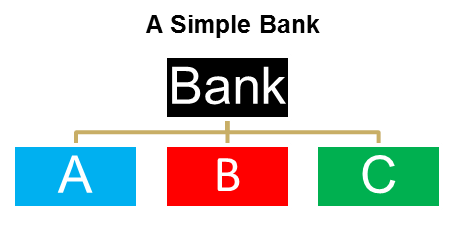
Bank's trading book
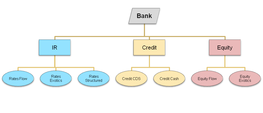
- The trading book hierarchy is well defined and stable over time
- Leaf nodes are the lowest level books, only containing individual trades, but not books
Diversification benefits
$\bs w = \sum_i \bs w_i$ is the company's whole portfolio
- $\bs w_i$ is the notional vector of the i-th business unit
- $\bs w_i$ could represent a single trade in the ultimate granularity
$c(\cdot)$ is a cost function of a portfolio:
- $c(\bs w) = c\left(\sum_i \bs w_i\right)$ is the cost of the whole company
- $c(\bs w_i)$ is the standalone cost of the i-th business unit of the company
- risk capital is the most important cost functions, such as VaR, IRC
For most risk capital metrics: $c\left(\sum_i \bs w_i\right) < \sum_i c(\bs w_i)$
- because of the diversification/hedging benefits
- total diversification benefits is therefore $\sum_i c(\bs w_i) - c\left(\sum_i \bs w_i\right)$
Allocation problem
How to divide the firm's total $c(\bs w)$ to individual business in an additive manner?
- allocated cost $\xi_i$: $c(\sum_i \bs w_i) = \sum_i \xi_i$ by definition.
- The core of the allocation problem is the fair distribution of diversification benefits
- $c(\bs w_i) - \xi_i$ is the diversification benefit allocated to the i-th business unit
- In practice, allocation runs all the way down to individual trades
Importance of allocation
Business performance is measured by return on capital (ROC)
- ROC is computed using allocated capital $\xi_i$, not the standalone capital $c(\bs w_i)$
- certain business is only viable as part of a bank as $\xi_i < c(\bs w_i)$
Business incentive is a critical consideration.
- allocated capital is actively managed by business heads
- allocation method directly affects trading desks' behaviour
- allocation method should incentivize risk reduction
- a business unit's action to reduce the firm's overall risk should also reduce its own allocation
Replacement cost
We use replacement cost as an example to illustrate allocation methods:
$$ \rc(\bs w) = \max(\bs w^T \bs v, 0)$$- $\bs v$ is the PV vector of all tradable instruments (per unit notional)
- $\bs w^T \bs v$ is the portfolio's total PV
Replacement cost is the aggregated PV of the portfolio against a particular counterparty, floored at 0
- part of the Basel 3 leveraged balance sheet capital
- it is a measure of MtM loss if the counterparty defaults
A simple example
A bank has only three trade against a counterparty, their PVs are: $ a = 12, b = 24, c = -24$
- The bank's total replacement cost is therefore: $$\rc(a + b + c) = \max(12 + 24 - 24, 0) = 12$$
- Diversification benefits: $$ \rc(a) + \rc(b) + \rc(c) - \rc(a+b+c) = 12 + 24 + 0 - 12 = 24$$
Standalone allocation
The simplest allocation strategy, allocation proportional to the standalone cost:
$$ \xi_i = \frac{c\left(\sum_i \bs w_i\right)}{\sum_i c(\bs w_i)} c(\bs w_i) $$Standalone allocation results:
| A | B | C | Total | |
|---|---|---|---|---|
| PV | 12 | 24 | -24 | 12 |
| Standalone RC | 12 | 24 | 0 | 36 |
| Standalone allocation | 4 | 8 | 0 | 12 |
- commonly used in practice
- not intrinsically additive, need the ad hoc scaling factor
- gives wrong business incentives (more on this later)
A model for fairness
In cooperative game theory, fairness is modeled by the following axioms:
- efficiency: allocations sum up to total
- symmetry: if two units' contribution are identical to any arbitrary subsets of units, their allocations are the same
- linearity: allocation of sums equals to the sum of allocations
- null: if a unit has no contribution to any subsets, it has 0 allocation
Shapley allocation is the only fair allocation method:
- A unit's allocation equals to the average of its marginal contributions over all possible permutations
Developed in 1960s, Sir L. Shapley received the 2012 Nobel prize.
Shapley allocation example
| Permutations | Cumulative RC | A | B | C |
|---|---|---|---|---|
| A=12, B=24, C=-24 | 12, 36, 12 | 12 | 24 | -24 |
| A=12, C=-24, B=24 | 12, 0, 12 | 12 | 12 | -12 |
| B=24, C=-24, A=12 | 24, 0, 12 | 12 | 24 | -24 |
| C=-24, B=24, A=12 | 0, 0, 12 | 12 | 0 | 0 |
| B=24, A=12, C=-24 | 24, 36, 12 | 12 | 24 | -24 |
| C=-24, A=12, B=24 | 0, 0, 12 | 0 | 12 | 0 |
| Averages | 10 | 16 | -14 |
Shapley allocation is additive by construction
- no need for any ad hoc scaling factors
Shapley allocation is computationally expensive
- requires Monte Carlo simulation for any non-trivial allocaiton problems
- e.g. the total number of permutation for 10 units is $10! = 3,628,800$
Associativity
Associativity means a top-down applicaiton of the allocation yields identical results as a bottom-up application:

Neither standalone nor Shapley allocation is associative:
| allocation to [A] | allocation to [BC] | |
|---|---|---|
| Top-down | 12 | 0 |
| Standalone bottom-up | 4 | 8 |
| Shapley bottom-up | 10 | 2 |
Associativity is critical in practice:
- Without it, the allocation algorithm is vulnerable to manipulations via trade rebooking.
The direction of attack:
- Tweak the Shapley allocation to make it associative
Aumann-Shapley allocation
A continuous limit of the Shapley allocation with allocation units being trades with infinitesimal notionals.
$$\bs u^T = \int_0^1 \frac{\partial c(q\bs w)}{\partial (q \bs w)} dq \iff u_k = \int_0^1 \frac{\partial c(q\bs w)}{\partial (q w_k)} dq $$- $\bs u$ is the allocation per unit notional of instruments
- the allocation to individual trades in the i-th unit are $\bs u \odot \bs w_i$
- the allocation to a portfolio is therefore $\xi_i = \bs u^T \bs w_i$.
- Associative by construction: inherited from vector summation
A-S allocation is much more efficient to compute than Shapley allocation.
The big blender
Conceptually the A-S allocation, $\bs u^T = \int_0^1 \frac{\partial c(q\bs w)}{\partial (q \bs w)} dq $, is a big blender:

- all organizational information are lost
- the allocation is computed from a homogenous soup of trades
Additivity of Aumann-Shapley
The A-S allocation is additive by construction:
$$\begin{array} \\ \sum_i \xi_i &= \sum_i \bs u^T \bs w_i = \bs u^T \bs w \\ &= \int_0^1 \frac{\partial c(q\bs w)}{\partial (q \bs w)} \bs w \; dq = \int_0^1 \frac{\partial c(q\bs w)}{\partial (q \bs w)} \frac{\partial (q \bs w)}{\partial q} \; dq \\ &= \int_0^1 d c(q\bs w) = c(\bs w) - c(\bs 0) \end{array}$$- it is customary to define $c(\bs 0) = 0$, ie, empty portfolio should have zero risk or capital cost.
Euler allocation
If the cost function is homogeneous, ie, $c(q \bs w) = q c(\bs w)$, the A-S allocation reduces to the Euler allocation:
$$ \bs u^T = \int_0^1 \frac{\partial c(q\bs w)}{\partial (q \bs w)} dq = \int_0^1 \frac{\partial c(\bs w)} { \partial \bs w} dq = \frac{ \partial c(\bs w)} {\partial \bs w} $$- In practice, most risk capital metrics are homogeneous
- Euler allocation is by trades' marginal contribution
- A-S/Euler allocation are computationtally efficient
- no need for Monte Carlo
Euler allocation of replacement cost
$$ \bs u^T = \frac{\partial \rc(\bs w)}{\partial \bs w} = \frac{\partial \max(\bs w^T \bs v, 0)}{\partial \bs w} = \ind(\bs w^T \bs v > 0) \bs v^T $$- $\frac{d}{dx} \max(x, 0) = \ind(x > 0)$, where $\ind(\cdot)$ is the indicator function
- the allocation is trade's MtM if the total PV is positive, otherwise 0
- it is indeed associative, the sum of allocation to B and C is 0
| A | B | C | Total | |
|---|---|---|---|---|
| A-S/Euler Allocation | 12 | 24 | -24 | 12 |
Perverse incentives
- A-S allocation could produce perverse incentives in practice
- A consequence of using infitesimal sized allocation unit
- Fairness depends on organization
Consider replacement cost of a bank with two trading desks X and Y:
| Day | X PV | Y PV | Banks RC | A-S/Euler Allocation |
|---|---|---|---|---|
| 1 | 12 | -10 | 2 | X=12, Y=-10 |
| 2 | 12 | -14 | 0 | X=0, Y=0 |
- Y gets penalized for reducing the bank’s overall RC to 0
- X gets a big reduction in capital allocation without doing anything
What's wrong with Shapley?
- The associativity is broken by two permutations that violates the bank’s organizational constraint.
- If we remove the two offending permutations from averaging, the Shapley allocation becomes associative.
| Permutations | Cumulative RC | A | B | C |
|---|---|---|---|---|
| A=12, B=24, C=-24 | 12, 36, 12 | 12 | 24 | -24 |
| A=12, C=-24, B=24 | 12, 0, 12 | 12 | 12 | -12 |
| B=24, C=-24, A=12 | 24, 0, 12 | 12 | 24 | -24 |
| C=-24, B=24, A=12 | 0, 0, 12 | 12 | 0 | 0 |
| B=24, A=12, C=-24 | 24, 36, 12 | 12 | 24 | -24 |
| C=-24, A=12, B=24 | 0, 0, 12 | 0 | 12 | 0 |
| Averages | of all | 10 | 16 | -14 |
| Averages | of admissibles | 12 | 15 | -15 |
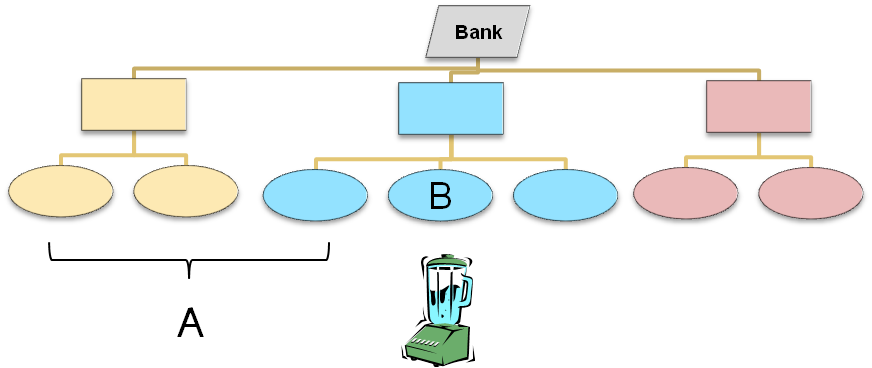
Constrained Shapley
A unit’s allocation equals its average incremental contribution, where the average is taken over all the permutations that are admissible under the organizational constraints.
Admissible permutations:
- All permutations are admissible for nodes with the same parent
- A branch (i.e. a node and all of its descendents) has to be permuted as a whole.
| Admissible Permutations | Inadmissible Permutations |
|---|---|
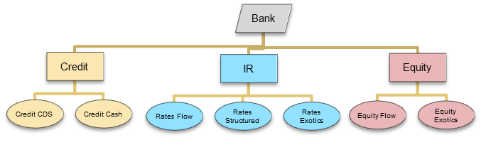 </br> </br> 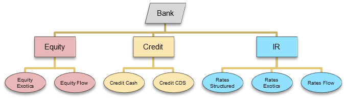 |
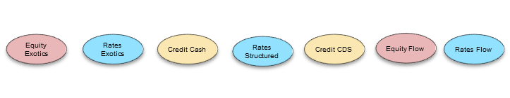 </br> </br>  |
- mixing trades from different leaf nodes also lead to inadmissible permutations
Correct incentives
The constrained Shapley is additive and associtive by construction, it gives the right incentives:
| Day | X PV | Y PV | Banks RC | C-Shapley Allocation |
|---|---|---|---|---|
| 1 | 12 | -10 | 2 | X=7, Y=-5 |
| 2 | 12 | -14 | 0 | X=6, Y=-6 |
- C-Shapley allocation gives the correct incentive for Y to reduce the overall bank’s RC.
C-Shapley features
Advantages of C-Shapley:
- additive and associative by construction
- gives the right business incentive
However, it is still computationally expensive:
- Impossible to exhaust all admissible permutations
- Monte Carlo permutation of large number of trades is challenging
Constrained Aumman-Shapley (CAS) is a continuous extension to C-Shapley:
- computationally efficient
- equivalent to C-Shapley on all nodes, different only in the allocation to individual trades
Business incentives
We take the following simple bank as an example:
The covariance matrix between the returns of three businesses are:
| A | B | C | |
|---|---|---|---|
| A | 1 | 0.65 | -0.9 |
| B | 0.65 | 1 | -0.9 |
| C | -0.9 | -0.9 | 1 |
We then scale the size of business C and see what happens to the firm's total VaR and its VaR allocations.
Allocation comparison


- Yellow region: increasing C reduces firm's overall VaR
- Standalone allocation failed to recognize and reward hedges
- Euler allocation failed to distribute diversification benefits
- Euler allocation is unstable
- Only C-S/CAS recognizes the main driver of the risk
Allocation summary
| Criteria | C-S/CAS | A-S/Euler | Shapley | Standalone |
|---|---|---|---|---|
| Associativity | yes | yes | no | no |
| Negative allocations for hedges | yes | yes | yes | no |
| Stability | good | poor | good | best |
| Predict marginal changes | good | best | good | poor |
| Distribute diversification benefits | yes | no | yes | yes |
| Recognize main risk driver | best | good | best | poor |
| Computational speed | good | good | poor | best |
C-Shapley/CAS allocation:
- stands out with the best set of features
- a candidate for universal risk capital allocation method
- applicable to a wide variety of risk capital metrics in banks
- applicable to the risk allocations of multiple trading strategies
Achieve the impossible
Change allocation methodology is almost mission impossible:
- zero-sum: a desk's gain is another desk's loss
- it affects the interests and livelihood of every business unit
- diffcult to build consensus amongst business units with conflicting interests
The only way to implement the change is to:
- establish a theoreticaly sound methodology that is impossible to argue against (C-Shapley/CAS)
- explain the methodology to every business unit, and ask business heads to document their objections
- "I don't like my allocation" is not a good objection
- the process takes time and effort
optional
Constrained Aumman-Shapley
Constrained Aumman-Shapley
- Constrained Aumman-Shapley (CAS) is a continuous generaization of the C-Shapley allocation
- Conceptually it is a small blender, that works within the organizational boundary
CAS allocation
The allocation per unit notional for trades in the portfolio B, conditioned on an admissible permutation is:
$$ \bs u^T(\bs w_B |\bs w_A) = \int_0^1 \frac{\partial c(\bs w_A + q\bs w_B)}{\partial (q \bs w_B)} dq $$The unconditional CAS allocation per unit notional for leaf node B is:
$$\bs u^T(\bs w_B) = \mathbb{E}\left[\bs u^T(\bs w_B | \bs w_A)\right]$$,
- the expectation is taken over all admissible permutations (i.e., all $\bs w_A$)
- the allocation for each trade in B is therefore $\bs u(\bs w_B) \odot \bs w_B$
- the allocation for the portfolio B is $\bs u^T(\bs w_B) \bs w_B$
CAS features
- Identical to C-Shapley for all nodes, only differ in individual trades
- Additive, for each admissible permutation:
- Associative, follows that of the C-Shapley
We will show later that CAS is:
- Computationally efficient
- Gives the right business incentives
Separability
The cost function is separable if
$$ \frac{\partial c(\bs w_A + q\bs w_B)}{\partial (q \bs w_B)} = \bs a^T(\bs w_A + q\bs w_B) S $$- $\bs a$ is a vector of the portfolio level parameters only
- $S$ is a matrix that only depends on individual trade's characteristics
Vast majority of risk capital metrics are separable:
- VaR and VaR variants like IRC, CRM
- Expected shortfall
- Replacement cost
Separate replacement cost
$$\begin{array}{l} \frac{\partial }{\partial (q \bs w_B)} \rc(\bs w_A + q \bs w_B) &= \frac{\partial }{\partial (q \bs w_B)} \max\left((\bs w_A + q \bs w_B)^T \bs v, 0 \right) \\ &= \ind ((\bs w_A + q \bs w_B)^T \bs v > 0) \bs v^T \end{array}$$- $\ind \left((\bs w_A + q \bs w_B)^T \bs v > 0\right)$ is only a function of the portfolio PV
- $\bs v$ is a vector of individual instrument's PV (per unit notional)
Efficiency and separability
For separable metrics, CAS allocation reduces to:
$$\mathbb{E}\left[\bs u^T(\bs w_B | \bs w_A)\right] = \mathbb{E}\left[\int_0^1 \frac{\partial c(\bs w_A + q\bs w_B)}{\partial (q \bs w_B )} dq \right] = \mathbb{E}\left[\int_0^1 \bs a^T(\bs w_A + q\bs w_B) dq \right] S $$- Being independent of $\bs w_A$ or $q$, $S$ can be pulled out of the expectation.
With separability, CAS allocation is extremely efficient:
- Simulate $\bs a(\bs w_B) = \mathbb{E}\left[\int_0^1 \bs a(\bs w_A + q\bs w_B) dq\right]$
- only sample leaf nodes' permutations
- no need to permute and track individual trades
- many orders of magnitude faster, millions of trades vs. thousands of leaf nodes
- The product $\bs a^T(\bs w_B) S$ can be done cheaply as a second step
Value at Risk
Value at risk (VaR) is a quantile measure of the portfolio's risk.
- If a portfolio's 10-day 99% VaR is \$10M, then the probabilty for the portfolio to lose more than \$10M in 10 days is 1%.
- It is the most important and widely quoted risk management metric
Mathematically VaR is a quantile measure: $$\renewcommand{rv}{\tilde{\bs v}}$$
$$ \mathbb{P}[\bs w^T \rv > \text{VaR}_\alpha] = \alpha $$- VaR is communicate as a positive number despite being a loss
- We write $\text{VaR} < 0$ and use $|\text{VaR}|$ explicitly when needed
- $\alpha$ is the quantile, like 99%
- $\bs w$ is the portfolio's notional vector of instruments,
- $\rv$ is the PV change of a unit notional instrument over the 10-day period, it is a random vector
- The above equation explicitly defined a $\text{VaR}_\alpha(\bs w)$ function
Computing VaR:
- Historical simulation: replay historical 10-day returns of all risk factors on today's portfolio
- Model simulation: build risk factor models using historical data and simulate many scenarios from the model
Marginal contribution to VaR:
A useful relationship: $$ \frac{\partial \v}{\partial \bs w} = \mathbb{E}[\rv^T | \bs w^T \rv = \v] $$
which can be derived as:
$$\small \begin{array} \\ 0 &= \frac{\partial}{\partial \bs w} \mathbb{P}\left[\bs w^T \rv > \v \right] = \frac{\partial}{\partial \bs w} \mathbb{E}\left[\ind(\bs w^T \rv - \v > 0)\right] \\ &= \mathbb{E}\left[\frac{\partial}{\partial \bs w} \ind (\bs w^T \rv - \v > 0)\right] = \mathbb{E}\left[ \delta (\bs w^T \rv - \v) (\rv^T - \frac{\partial \v}{\partial \bs w})\right] \\ &= \mathbb{E}\left[\rv^T - \frac{\partial \v}{\partial \bs w} \vert \bs w^T \rv = \v\right] = \mathbb{E}\left[\rv^T \vert \bs w^T \rv = \v\right] - \frac{\partial \v}{\partial \bs w} \end{array}$$- $\ind(x)$ is the indicator function, $\frac{d}{dx}\ind(x>0) = \delta(x)$
- $\delta(x)$ is the Dirac's delta function, with $\intr f(x) \delta(c) dx = f(c)$
Separability of VaR
The VaR can be written in a separable form using its marginal contribution:
$$\begin{array}{l} \frac{\partial \v (\bs w_A + q \bs w_B)}{\partial (q \bs w_B)} &= \mathbb{E}[\rv^T | (\bs w_A + q\bs w_B)^T \rv = \v] \\ &= \bs k^T(\bs w_A + q\bs w_B) V \end{array}$$The first equality can be proved similarly using the steps in the previous slide.
- $\bs k^T$ is a Gaussian Kernel
- $V$ is a matrix of the historical 10-day PnL for all the individual trades