Review of Linear Algebra
Richard Feynman: In fact, mathematics is, to a large extent, invention of better notations.
Vector
- Is a set of elements, which can be real or complex:
$\renewcommand{bs}{\boldsymbol}$
$$ \begin{matrix} \bs u = \left( \begin{matrix} u_1 \\ u_2 \\ \vdots \\ u_n \end{matrix} \right) \hspace{2cm} \bs v = \left( \begin{matrix} v_1 \\ v_2 \\ \vdots \\ v_n \end{matrix} \right) \end{matrix} $$
Basic vector operations
- Vector addition: $\bs{w = u + v}$
- Scalar multiplication: $\bs w = a \bs u$, where $a$ is a scalar
Notation
We use the following notation throughout the class:
- column vector: $\bs {u, v, x, \beta}$
- row vector: $\bs u^T, \bs v^T, \bs x^T, \bs \beta^T$
- scalar: $a, b, \alpha, \beta$
- matrix: $A, B, P$
- random variables: $\tilde a, \tilde{\bs u}, \tilde{\bs v}^T$
Vector addition
- Associativity: $\bs{u + (v + w) = (u + v) + w}$
- Commutativity: $\bs{u + v = v + u}$
- Identity: $\bs{v + 0 = v}$ for $\forall \bs{v}$
- Inverse: for $\forall \bs{v}$, exists an $-\bs{v}$, so that $\bs{v + (-v) = 0}$
- Distributivity: $a \bs{(u + v)} = a \bs{u} + a \bs v, (a+b) \bs v = a \bs v + b \bs v$
Scalar multiplication
- Associativity: $a(b \bs v) = (ab)\bs v$
- Identity: $1 \bs v = \bs v$, for $\forall \bs v$
Linear combination
- $\bs v = a_1 \bs v_1 + a_2 \bs v_2 + ... + a_n \bs v_n$
- Linear combinations of vectors form a subspace $\Omega_v = \text{span}(\bs{v_1, v_2, ... v_n}) \subset \Omega$
- Linear independence: $\bs {v = 0} \iff a_k = 0$ for $\forall k$
- Basis: any set of linearly independent $\bs v_i$ that spans $\Omega_v$
- Dimension of $\Omega_v$ is the number of vectors in (any of) its basis
Inner product
- $\langle \bs u, a \bs v_1 + b \bs v_2 \rangle = a \langle \bs{u, v_1} \rangle + b \langle \bs{u, v_2} \rangle$
- $\langle \bs{u, v} \rangle = \langle \bs{v, u} \rangle^c$
- $\langle \bs{u, u} \rangle \ge 0$
- $\langle \bs{u, u} \rangle = 0 \iff u = 0$
- $\bs {u, v}$ orthogonal if $\langle \bs{u, v} \rangle = 0$
Dot product
A special case of inner product:
- the standard inner product: $\bs{u \cdot v} = \sum_{k=1}^n u_k^c v_k$
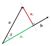
- the magnitude of a vector $\bs b$ is $\vert b \vert = \sqrt{\bs b \cdot \bs b}$
- the projection of vector $\bs a$ to the direction of vector $\bs b$ is: $ a_1 = \frac{\bs a \cdot \bs b}{\vert b \vert} = \vert \bs a \vert \cos(\theta) $
Matrix
- Represents a linear response to multiple input factors:
$$ \overset{\text{Outputs}}{\longleftarrow}\overset{\downarrow \text{Inputs}} {\begin{pmatrix} a_{11} & a_{12} & . & a_{1n} \\ a_{21} & a_{22} & . & a_{2n} \\ . & . & . & \\ a_{m1} & a_{m2} & . & a_{mn} \end{pmatrix}} $$
- Matrix addition and scalar multiplication are element wise, similar to those for vectors
Matrix multiplication
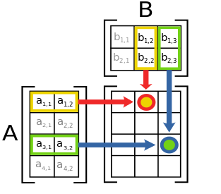
$$\begin{array} \\ \bs u = A \bs v &\iff u_i = \sum_{j=1}^{n} a_{ij}v_j \\ C = AB &\iff c_{ij} = \sum_{k=1}^{n} a_{ik}b_{kj} = a_i \cdot b_j \end{array}$$
Matrix represents linear transformation
Linear function on vectors:
- $L(\bs{u + v}) = L(\bs u) + L(\bs v)$
- $L(a \bs v) = a L(\bs v)$
Any linear transformation between finite dimensional vector space can be represented by a matrix multiplication, therefore we can write $L \bs u$ instead of $L(\bs u)$.
Properties of linear transformation
- Associativity: $A(BC) = (AB)C$
- Distributivity:
- $A(B+C) = AB + AC$
- $(B+C)A = BA + CA$
- $\alpha (A+B) = \alpha A + \alpha B$
- But not commutative: $AB \ne BA$
$\renewcommand{id}{I}$
Matrix definitions
- Identity matrix $\id$: $\id A = A \id = A$
- $A^T$ is the transpose of $A$: $a^T_{ij} = a_{ji}$
- Symmetric matrix: $A = A^T$
- $A^*$ is the adjoint of $A$: $a^*_{ij} = a_{ji}^c$
- real matrix: $A^T = A^*$
- self-adjoint (Hermitian) matrix: $A = A^*$
- Inverse matrix: $AA^{-1} = A^{-1}A = \id$
- Orthogonal matrix: $A^T = A^{-1} \iff AA^T = \id$
LU Factorization
Factorize: to resolve into factors.
Linear system
- In matrix form, a linear system is $A \bs {x = y}$
- It has a unique solution if $A$ is a full rank square matrix
a = sp.Matrix([[2, 1, -1], [-6, -2, 4], [-2, 1, 2]])
y = sp.Matrix([8, -22, -3])
X = sp.MatrixSymbol('x', 3, 1)
x1, x2, x3 = sp.symbols('x_1, x_2, x_3')
x = sp.Matrix([x1, x2, x3])

fmt.displayMath(a, fmt.joinMath('=', x, y), sep="", pre="\\scriptsize ")
Gaussian elimination
Eliminate the $x_1$ terms using the first row, this operation is a linear transformation:
A = sp.MatrixSymbol('A', 3, 3)
L1 = sp.MatrixSymbol('L_1', 3, 3)
L2 = sp.MatrixSymbol('L_2', 3, 3)
l1 = sp.eye(3)
l1[1, 0] = -a[1, 0]/a[0, 0]
l1[2, 0] = -a[2, 0]/a[0, 0]

fmt.displayMath(L1*a, fmt.joinMath('=', x, L1*y), "\;,\;\;", l1*a, fmt.joinMath('=', x, l1*y), sep="",
                pre="\\scriptsize ")
Use the 2nd equation (row) to eliminate the $x_2$ terms:
l2 = sp.eye(3)
a2 = l1*a
y2 = l1*y
l2[2, 1] = -a2[2, 1]/a2[1, 1]
u = l2*a2
fmt.displayMath(L2*a2, fmt.joinMath('=', x, L2*y2), "\;,\;", u, fmt.joinMath('=', x, l2*y2),
                sep="", pre="\\scriptsize ")
the $L_1$ and $L_2$ are both lower triangular matrices
Ui = sp.MatrixSymbol('U^{-1}', 3, 3)
U = sp.MatrixSymbol('U', 3, 3)
L = sp.MatrixSymbol('L', 3, 3)
fmt.displayMath(fmt.joinMath('=', L1, l1), fmt.joinMath('=', L2, l2), fmt.joinMath('=', U, u),
                pre="\\scriptsize ")
The resulting matrix $U = L_2L_1A$ is upper triangular
LU factorization
The triangular matrix is easy to invert by variable replacement
y3 = l2*y2
a3 = l2*a2
ui = a3.inv()
fmt.displayMath(fmt.joinMath('=', Ui, ui), "\;,\;", fmt.joinMath('=', x, Ui),
                fmt.joinMath('=', l2*y2, ui*y3), sep="\;", pre="\\scriptsize ")
Now we can group $L = L_1^{-1}L_2^{-1}$ and obtain the LU factorization
$$L_2 L_1 A = U \iff A = L_1^{-1} L_2^{-1} U \iff A = LU $$
- $U$ is a upper triangular matrix.
- There can be infinite numbers of LU pairs, the convention is to keep the diagonal elements of $L$ matrix 1.
l =  l1.inv()*l2.inv()
fmt.displayMath(fmt.joinMath('=', L, l), fmt.joinMath('=', U, a3), fmt.joinMath('=', L*U, l*a3),
                pre="\\scriptsize ")
- The LU factorization is the matrix representation of Gaussian elimination
- LU factorization can be used to compute matrix inversion
- triangular matrix can be inverted by simple substitution
Pivoting
The Gaussian elimination does not work if there are 0s in the diagonal of the matrix.
- The rows of the matrix can be permuted first, so that the diagonal elements have the greatest magnitude.
- Permuting rows is a linear operation, thus it can be expressed as a Matrix $P$
$$ A = P \cdot L \cdot U $$
where the $P$ matrix represents the row permutation. The permutation (pivoting) also improve the numerical stability:
from scipy.linalg import lu

def displayMultiple(fs) :
    tl=map(lambda tc: '$' + sp.latex(tc) + '$',fs)
    r = '''
  <table border="0"><tr>'''
    for v in tl :
        r += "<td>" + v + "</td>"
    r += "</tr></table>"
    return r

a = sp.Matrix([[0, 3, 1, 2], [4, 0, -3, 1], [-3, 1, 0, 2], [9, 2, 5, 0]])
p, l, u = map(lambda x: sp.Matrix(x), lu(a))
Pi = sp.MatrixSymbol('P^{-1}', 4, 4)
A = sp.MatrixSymbol('A', 4, 4)
P = sp.MatrixSymbol('P', 4, 4)
fmt.displayMath(fmt.joinMath('=', A, a), fmt.joinMath('=', P, p), pre="\\scriptsize ")
fmt.displayMath(sp.Eq (Pi*A, p.inv()*a), pre="\\scriptsize ")
Cholesky Decomposition
a.k.a Cholesky Factorization
Covariance matrix
The most important and ubiquitous matrix in quant Finance,
- given random factors $\bs{\tilde r} = [r_1, ..., r_n]^T$ and their expectation: $\bar{\bs r} = \mathbb{E}[\bs {\tilde r}]$
The covariance matrix is:
$$V = \mathbb{E}[(\bs {\tilde r} - \bar{\bs r})(\bs {\tilde r} - \bar{\bs r})^T] = \mathbb{E}[\bs{\tilde r} \bs{\tilde r}^T] - \bar{\bs r}\bar{\bs r}^T $$
- The element $(i, j)$ in $V$ is: $\text{cov}(r_i, r_j) = \rho_{ij} \sigma_i \sigma_j$.
Covariance of linear combinations of factors:
$$\begin{array}{l} \text{cov}(\bs x^T \bs r, \bs y^T \bs r) &= \mathbb{E}[(\bs x^T \bs r)(\bs r^T \bs y)] - \mathbb{E}[\bs x^T \bs r]\mathbb{E}[\bs r^T \bs y]\\ &= \bs x^T \mathbb{E}[\bs r \bs r^T] \bs y - \bs x^T \bar{\bs r}\bar{\bs r}^T \bs y = \bs x^T V \bs y \end{array}$$
Correlation matrix
$\renewcommand{Sigma}{\mathcal{S}}$
- $C = (\rho_{ij})$ is the co-variance matrix of the normalized factors $\bs {\tilde s} = [\frac{r_1}{\sigma_1}, ..., \frac{r_n}{\sigma_n}]^T$
- $V = \Sigma C \Sigma $, where $\Sigma$ is a diagonal matrix of $\sigma_i$
- all elements in a correlation matrix are within [-1, 1]
Symmetric positive definite (SPD)
Positive definite:
- Matrix $A$ is positive definite if $\bs x^T A \bs x > 0$ for $\forall \bs{x \ne 0}$
- Matrix $A$ is semi positive definite if $\bs x^T A \bs {x \ge 0}$ for $\forall \bs{x \ne 0}$
- Positive definite does not imply every element in the matrix is positive
Both covariance and correlation matrices are symmetric (semi) positive definite (SPD):
- $\bs x^T V \bs x = \text{cov}[\bs x^T \bs {\tilde r},\bs x^T \bs {\tilde r}] = \text{var}[\bs x^T \bs {\tilde r}] \ge 0$
- $\bs x^T C \bs x = \text{cov}[\bs x^T \bs {\tilde s},\bs x^T \bs {\tilde s}] = \text{var}[\bs x^T \bs {\tilde s}] \ge 0$
Example: weekly price and returns
import pandas as pd
f3 = pd.read_csv('data/f3.csv', parse_dates=[0]).set_index('Date').sort_index()

fig = figure(figsize=[12, 4])
ax1 = fig.add_subplot(121)
f3.plot(title='Historical Prices', ax=ax1);

weeks_in_year = 52. #business weeks per year

ax2 = fig.add_subplot(122)
r = np.log(f3).diff()
r.plot(title='Historical Returns', ax=ax2);

Correlation and covariance matrix of weekly returns:
cm = r.corr()
cv = r.cov()

fmt.displayDFs(cm, cv*weeks_in_year, headers=['Correlation', 'Covariance'], fontsize=4, fmt="4f")
- Does it make sense to compute the covariance and correlation matrix of the price levels?
Cholesky decomposition
If $A$ is symmetric semi positive definite (SPD) matrix
- $A$ can be decomposed as $A = LL^T$, where $L$ is lower triangle
- In another word, the $U = L^T$ in $A$'s LU decomposition
- $L$ can be viewed as the "square root" of $A$
Cholesky decomposition is not unique if the matrix is semi positive definite, but unique when it is positive definite:
- The rank is same between $L$ and $A$
- Beware that $A = LL^T \neq L^TL$
Examples of Cholesky decomposition:
Previous correlation matrix:
lcm = np.linalg.cholesky(cm)
lcv = np.linalg.cholesky(cv)
fmt.displayMath(sp.Matrix(lcm).evalf(4),
                fmt.joinMath('=', sp.Matrix(lcm.T).evalf(4), sp.Matrix(lcm.dot(lcm.T)).evalf(4)),
                sep="", pre="\\tiny")
Previous covariance matrix:
fmt.displayMath(sp.Matrix(lcv).evalf(3),
                fmt.joinMath('=', sp.Matrix(lcv.T).evalf(3), sp.Matrix(lcv.dot(lcv.T)).evalf(3)),
                sep="", pre="\\tiny")
Recursive algorithm
A SPD matrix $A$ and its Cholesky decomposition $L$ can be partitioned as:
s_A, a11, A12, A21, A22 = sp.symbols("A, a_{11} A_{21}^T A_{21} A_{22}")
s_L, s_LT, l11, L12, L12T, L22, L22T = sp.symbols("L L^T l_{11} L_{21} L_{21}^T L_{22} L_{22}^T")

A = sp.Matrix([[a11, A12], [A21, A22]])
L = sp.Matrix([[l11, 0], [L12, L22]])
LT = sp.Matrix([[l11, L12T], [0, L22T]])

fmt.displayMath(fmt.joinMath('=', s_A, A), fmt.joinMath('=', s_L, L), fmt.joinMath('=', s_LT, LT)
               , pre='\\scriptsize')
From $A = LL^T$:
fmt.displayMath(fmt.joinMath('=', A, L*LT), pre='\\scriptsize')
We immediately have:
fmt.displayMath(fmt.joinMath('=', l11, sp.sqrt(a11)), fmt.joinMath('=', L12,  A21/l11),
                fmt.joinMath('=', A22 - L12*L12T, L22*L22T), pre='\\scriptsize')
Note that $L_{22}$ is the Cholesky decomposition of the smaller matrix of $A_{22} - \frac{1}{a_{11}}A_{21}A_{21}^T$.
Correlated Brownian motion
Ubiquitous in quantitative Finance
- The most common processes for asset prices and risk factors
Example: correlated n-dimensional Geometric Brownian motion:
$$ \frac{dx^k_t}{x^k_t} = u^k dt + \sigma^k dw^k_t, \;\;\;\;dw_t^j\cdot dw_t^k = \rho_{jk} dt $$
In vector form: $$ d \bs x = X \bs u dt + X \Sigma d \bs w, \;\;\; d\bs w d\bs w^T = C dt$$
where $X$ is a diagonal matrix of $x_i$, and $\Sigma$ is a diagonal matrix of $\sigma_i$ and $C$ is the correlation matrix of $\rho_{ij}$
Draw correlated Brownians
Draw discretized version of $\delta \bs w = L \bs z \sqrt{\delta t}$
- where $\bs z$ is a vector of independent standard normal random variables
- $\mathbb{E}[\bs z] = \bs 0$, $\mathbb{E}[\bs z \bs z^T] = I$
- $L$ is the Cholesky decomposition of the correlaton matrix $C = LL^T$
$\delta \bs w$ have the desired correlation: $$\mathbb{E}[\delta \bs w \delta \bs w^T] = \mathbb{E}[L \bs z \bs z^T L^T] \delta t = L \mathbb{E}[\bs z \bs z^T] L^T \delta t = LL^T \delta t = C \delta t$$
Equivalently, we can draw $\Sigma \delta \bs w = (\Sigma L) \bs z\sqrt{\delta t}$, where
- $\Sigma L$ is the Cholesky decomposition of the covariance matrix $$ C = LL^T \iff V = \Sigma C \Sigma = \Sigma L (\Sigma L)^T $$
Simulated paths
# the code below ignores the drifts and its correction

nweeks = 1000
e = np.random.normal(size=[3, nweeks])
dw = (lcm.dot(e)).T
ts = np.arange(nweeks)/weeks_in_year

dws = dw*np.diag(cv)
wcm = np.exp(np.cumsum(dws, 0))

figure(figsize=[12, 4])
subplot(1, 2, 1)

stdev = np.sqrt(np.diag(cv))

dw = (lcm.dot(e)).T
dws = dw*stdev
wcm = np.exp(np.cumsum(dws, 0))
plot(ts, wcm)
xlabel("Year")
legend(cm.index, loc='best');
title('$L \epsilon$')

subplot(1, 2, 2)
dw2 = (lcm.T.dot(e)).T
dws2 = dw2*stdev
wcm = np.exp(np.cumsum(dws2, 0))
plot(ts, wcm)
xlabel("Year")
legend(cm.index, loc='best');
title(('$L^T \epsilon$'));

$L \bs \epsilon$ and $L^T \bs \epsilon$ are different, gives different correlation
df1 = pd.DataFrame(np.corrcoef(dws.T), columns=cm.index, index=cm.index)
df2 = pd.DataFrame(np.corrcoef(dws2.T), columns=cm.index, index=cm.index)

fmt.displayDFs(df1, df2, headers=['$L \epsilon$', '$L^T \epsilon$'], fontsize=4)
Big correlation/covariance matrices
In practice, we work with thousands of risk factors
- Correlation matrix is easier to maintain than the covariance matrix, because it is "normalized"
Very difficult to keep large correlation matrices semi positive definite (SPD)
- Size of a few thousands is the practical limit
- Small changes in few values can invalidate the whole matrix
- Adding new entries can be extremely difficult
Dimensionality reduction is required when dealing with very large number of factors.
Complexity
Complexity of a numerical algorithm is stated in the order of magnitude, often in the big-O notation:
- binary search $O(\log(n))$
- best sorting algorithm: $O(n \log(n))$
Most common numerical linear algebra algorithms are of complexity of $O(n^3)$
- matrix multiplication: $n^2$ elements in output, each element takes $O(n)$
- LU decomposition: $n$ diagonal elements, to zero-out each column costs $O(n^2)$
- Cholesky decomposition: $n$ recursive steps, each takes $O(n^2)$
Matrix Calculus
Morpheus: The Matrix is a system, Neo.
Scalar function
$$f(\bs x) = f(x_1, ..., x_n)$$
- Derivative to vector (Gradient): $\frac{\partial f}{\partial \bs x} = \nabla f = [\frac{\partial f}{\partial x_1}, ..., \frac{\partial f}{\partial x_n}]$
- Note that $\frac{\partial f}{\partial \bs x}$ is always a row vector, whenever the vector or matrix appears in the denominator of differentiation, the result is transposed.
- Some time we use the notation: $\frac{\partial f}{\partial \bs x^T} = \left(\frac{\partial f}{\partial \bs x}\right)^T $ to denote a column vector.
Vector function
$$\renewcommand{p}{\partial}\bs y(\bs x) = [y_1(\bs x), ..., y_n(\bs x)]^T$$
- Derivative to vector (Jacobian matrix): $\frac{\partial \bs y}{\partial \bs x} = \left[\frac{\partial{y_1}}{\partial \bs x}, \frac{\partial{y_2}}{\partial \bs x}, \cdots, \frac{\partial{y_n}}{\partial \bs x} \right]^T$
- $\frac{\partial \bs y}{\partial \bs x}$ is a matrix of $\bs y$ rows and $\bs x$ columns
- $\frac{\partial \bs y}{\partial \bs x}\frac{\partial \bs x}{\partial \bs y} = \id$, even when $\bs x$ and $\bs y$ are of different dimension.
- sometime we use the following notation: $\frac{\partial \bs y}{\partial \bs x^T} = \left(\frac{\partial \bs y}{\partial \bs x}\right)^T$
- Derivative to scalar: $\frac{\partial \bs y}{\partial z} = [\frac{\partial y_1}{\partial z}, \cdots, \frac{\partial y_n}{\partial z}]^T$
- remains a column vector
Vector differentiation cheatsheet
- $A, a, b, \bs c$ are constants (ie, not functions of $\bs x$)
- $\bs {u=u(x), v=v(x)}, y=y(\bs x)$ are functions of $\bs x$
- $O$ is the zero matrix, $I$ is the identity matrix
| Expression | Results | Special Cases |
|---|---|---|
| $\frac{\p(a \bs u + b \bs v)}{\p \bs x}$ | $a \frac{\p{\bs u}}{\p \bs x} + b\frac{\p{\bs v}}{\p \bs x}$ | $\frac{\p{\bs c}}{\p \bs x} = O, \frac{\p{\bs x}}{\p \bs x} = \id$ |
| $\frac{\p{A \bs u}}{\p \bs x}$ | $A\frac{\p{\bs u}}{\p \bs x}$ | $\frac{\p{\bs A x}}{\p \bs x} = A, \frac{\p{\bs x^T A}}{\p \bs x} = A^T$ |
| $\frac{\p{y \bs u}}{\p \bs x}$ | $y \frac{\p{\bs u}}{\p \bs x} + \bs u \frac{\p{y}}{\p \bs x}$ | - |
| $\frac{\p \bs{u}^T A \bs v}{\p \bs x} $ | $\bs u^T A \frac{\p{\bs v}}{\p \bs x} + \bs v^T A^T \frac{\p{\bs u}}{\p \bs x} $ | $\frac{\p \bs{x}^T A \bs x}{\p \bs x} = \bs x^T (A + A^T) $, $\frac{\p \bs{u^Tv}}{\p \bs x} =\bs{u}^T\frac{\p \bs{v}}{\p \bs x} + \bs{v}^T\frac{\p \bs{u}}{\p \bs x}$ |
| $\frac{\p{\bs g(\bs u})}{\p \bs x}$ | $\frac{\p{\bs g}}{\p \bs u} \frac{\p{\bs u}}{\p \bs x} $ | $\frac{\p \bs y}{\p \bs x}\frac{\p \bs x}{\p \bs y} = \id$ , $\frac{\p \bs z}{\p \bs y}\frac{\p \bs y}{\p \bs x} \frac{\p \bs x} {\p \bs z}= \id$, multi-step chain rules. |
- Similar to univariate calculus, a compact notation for multivariate calculus
- Replace $A^T$ by $A^*$ for complex matrix
Portfolio optimization
Powerful mean/variance portfolio theory can be expressed succinctly using linear algebra and matrix calculus.
Suppose there are $n$ risky assets on the market, with random return vector $\tilde{\bs r}$ whose covariance matrix is $V$,
- $\bs w$: a portfolio, its elements are values (dollar) invested in each asset
- $\bs w^T \tilde{\bs r}$ is the portfolio's P&L
- $\sigma^2 = \bs w^TV\bs w$: the variance of the portfolio P&L
Excess return forecast
- $\bs f = \mathbb{E}[\tilde{\bs r}] - r_0$ is a vector of excess return forecast of all risky assets
- $r_0$ is the risk free rate
- $\bs f$ is a view, which can be from:
- Fundamental research: earning forecasts, revenue growth etc
- Technical and quantitative analysis
- Your secret trading signal
Sharpe ratio
Sharpe ratio of a portfolio $\bs w$: $$s(\bs w) = \frac{\bs w^T \bs f}{\sqrt{\bs w^T V \bs w}}$$
Sharpe ratio is invariant under:
- portfolio scaling: $s(a \bs w) = s(\bs w)$
- leverage or deleverage: borrowing or lending money using the risk free asset
Portfolio optimization
Given the view $\bs f$, the optimal portfolio $\bs w$ to express the view is:
- minimize the variance of portfolio P&L (risk): $\bs w^TV\bs w$
- while preserving a unit dollar of excess P&L: $\bs w^T \bs f = 1$
which solves the portfolio $\bs w^*$ with the maximum Sharpe ratio under the view $\bs f$:
- $\bs w^*$ is a unique solution
- all portfolios with optimal Sharpe ratio have the same risky asset mix
- No need to constrain the total value because Sharp ratio is invariant by scaling the portfolio.
Why we take the covariance matrix $V$ as a constant, but treat expected return $\bs f$ as a variable?
Characteristic portfolio
The optimal portfolio can be solved analytically using Lagrange multiplier and matrix calculus:
$$\begin{eqnarray} l &=& \bs w^TV \bs w - 2 \lambda (\bs f^T \bs w - 1) \\ \frac{\partial l}{\partial \bs w^T} &=& 2 V \bs w - 2 \lambda \bs f = \bs 0 \\ \bs w &=& \lambda V^{-1} \bs f \end{eqnarray}$$
plug it into $\bs f^T \bs w = 1$:
$$ \bs f^T(\lambda V^{-1} \bs f) = 1 \iff \lambda = \frac{1}{\bs f^T V^{-1} \bs f}$$ $$\bs w^*(\bs f) = \frac{V^{-1}\bs f}{\bs f^T V^{-1} \bs f} \propto V^{-1}\bs f$$
$\bs w^*(\bs f)$ is also known as the characteristic portfolio for the forecast $\bs f$.
Relativity of return forecast
The optimal portfolio unchanged if $\bs f$ is scaled by a scalar $a$:
$$\bs w^*(a\bs f) = \frac{1}{a} \bs w^*(\bs f)$$
- $\bs w^*$ and $\frac{1}{a} \bs w^*$ defines the same risky asset mix, with identical Sharpe ratio
Therefore, only the relative sizes of excess returns are important
- e.g. excess return forecast of [1%, 2%] and [10%, 20%] of two assets would result in identical optimal (characteristic) portfolio
Benchmark portfolio and $\bs \beta$
Benchmark portfolio $\bs w_b$ is usually an index portfolio to measure the performance of active portfolio management.
- The beta of a portfolio $\bs w$ to the benchmark is $$\frac{\text{cov}(\bs w^T \tilde{\bs r}, \bs w_b^T \tilde{\bs r})}{\sigma_b^2} = \frac{\bs w^T V \bs w_b}{\sigma_b^2} = \bs w^T \bs \beta_b$$
- Define $\bs \beta_b = \frac{V\bs w_b}{\sigma^2_b} $, the vector of individual assets' betas
- $\bs w_b^T \bs \beta_b = \frac{\bs w_b^T V\bs w_b}{\sigma^2_b} = {1}$, the benchmark portfolio itself has a unit beta
$\bs w_m$ is the market portfolio, as defined in CAPM
- $\bs \beta_m = \frac{V\bs w_m}{\sigma^2_m}$: the betas vector to the market portfolio $\bs w_m$
Important characteristic portfolios
Identical returns: $\bs f \propto \bs e = [1, 1, ...., 1]^T$:
- A naive view that all assets have the same excess returns (zero information)
- $\bs e^T\bs w = 1$ means it is a portfolio of \$1 fully invested in risky assets
- $\bs w_e = \frac{V^{-1}\bs e}{\bs e^TV^{-1}\bs e}$ has the minimum variance of those fully-invested
Beta to a benchmark portfolio: $\bs f \propto \bs \beta_b = \frac{V\bs w_b}{\sigma_b^2}$:
- $\bs \beta_b^T \bs w_b = 1$ means the portfolio has a beta of 1 to the benchmark portfolio $\bs w_b$
- $\bs w_{\beta} = \frac{V^{-1}\bs \beta_b}{\bs \beta_b^T V^{-1}\bs \beta_b} = \frac{\bs w_b}{\bs{\beta_b^T w_b}} = \bs w_b$, i.e., the benchmark portfolio itself
- the benchmark portfolio itself is optimal amongst those with unit beta.
Portfolio optimization example
Given the following covariance matrix estimates and excess return forecasts:
er = np.array([.05, .02, .01]).T
flat_r = np.array([.01, .01, .01]).T
df_er = pd.DataFrame(np.array([er, flat_r]).T*100, columns=["Forcast (%)", "Naive(%)"], index = f3.columns).T


fmt.displayDFs(cv*1e4, df_er, fontsize=4, headers=['Covariance', 'Epected Excess Return'])
The (normalized) optimal portfolio for the given forecast is:
cvi = np.linalg.inv(cv)
w = cvi.dot(er.T)/er.T.dot(cvi).dot(er)
w = w/np.sum(w)
df_er.loc['Optimial Portfolio (O)', :] = w

w2 = cvi.dot(flat_r.T)/er.T.dot(cvi).dot(flat_r)
w2 = w2/np.sum(w2)
df_er.loc['Min Vol Portfolio (C)', :] = w2

fmt.displayDF(df_er[-2:], "4g", fontsize=4)
Efficient Frontier
The simulated Sharpe ratios of all $1 portfolios fully invested in risky assets:
- the optimal portfolio O has the optimal Sharpe Ratio
- the min Variance portfolio C has the smallest variance
- the line start from origin because we used excess return everywhere
rnd_w = np.random.uniform(size=[3, 10000]) - 0.5
rnd_w = np.divide(rnd_w, np.sum(rnd_w, 0))

rnd_r = er.dot(rnd_w)
rnd_vol = np.sqrt([p.dot(cv).dot(p.T) for p in rnd_w.T])

vol_o = sqrt(w.dot(cv).dot(w))
r_o = er.dot(w)
plot(rnd_vol, rnd_r, 'g.')
plot([0, 10*vol_o], [0, 10*r_o], 'k');
xlim(0, .06)
ylim(-.01, .08)

plot(vol_o, r_o, 'ro')
text(vol_o-.001, r_o+.003, 'O', size=20)
r_c = er.dot(w2)
vol_c = sqrt(w2.dot(cv).dot(w2))
plot(vol_c, r_c, 'r>')
text(vol_c-.002, r_c-.008, 'C', size=20);

legend(['Portfolios', 'Optimal Sharpe Ratio'], loc='best')

ylabel('Portfolio Expected Excess Return')
xlabel('Portfolio Return Volatility')
title('Sharpe Ratios of $1 portfolios');

Implied view of a portfolio
From any portfolio, we can back out its implied excess return forecast $\bs f$:
- Assuming the portfolio is mean variance optimal
- It is nothing but the betas to the portfolio
- Only meaningful in a relative sense as well
Consider the market portfolio: the market collectively believe that $\bs f \propto \bs \beta_m$:
$$\mathbb{E}[\tilde{\bs r}] - r_0 = \bs \beta_m \left(r_m - r_0\right)$$
- $r_m = \frac{\mathbb{E}[\bs w_m^T \bs {\tilde r}]}{\bs w_m^T \bs 1} $ is the market portfolio's expected return
- this is exactly the CAPM.
Estimate expected returns
Estimate expected return from historical data is difficult
- historical return is not a good indicator of future performance
- even if we assume it is, it requires very long history, ~500 years
The market implied return is a much better return estimate than historical data.
- This is the key insight of Black-Litterman
Implied views example
Suppose we are given the following portfolio:
w = np.array([10, 5, 5])
vb = w.dot(cv).dot(w)
ir = cv.dot(w)/vb

df = pd.DataFrame(np.array([w, ir])*100, index=["$ Position", "Implied Return %"],
                  columns = ["SPY", "GLD", "OIL"])
fmt.displayDF(df[:1], "4g", fontsize=4)
We can compute its implied return forecast as:
fmt.displayDF(df[1:], "2f", fontsize=4)
- note that these forecast are only meaningful in a relative sense
Does the investor really have so much confidence in OIL?
Norm and Condition
Robert Heinlein: Throughout history, poverty is the normal condition of man.
Ill-conditioned covariance matrix
The Mean-variance optimization is very powerful, but there are potential pitfalls in practice:
- Suppose we have the following covariance matrix and excess return forecast, then we can compute the optimal portfolio.
nt = 1000
es = np.random.normal(size=[2, nt])

rho = .999999
e4 = rho/np.sqrt(2)*es[0, :] + rho/np.sqrt(2)*es[1,:] + np.sqrt(1-rho*rho)*np.random.normal(size=[1, nt])
es = np.vstack([es, e4])

cor = np.corrcoef(es)
cor1 = np.copy(cor)
cor1[0, 1] = cor1[1, 0] = cor[0, 1] + .00002

sd = np.eye(3)
np.fill_diagonal(sd, np.std(r))
cov = sd.dot(cor).dot(sd.T)
cov1 = sd.dot(cor1).dot(sd.T)

e, v = np.linalg.eig(np.linalg.inv(cov))
er = v[:, 2]/10

df_cov = pd.DataFrame(cov*1e4, index=f3.columns, columns=f3.columns)
df_cov1 = pd.DataFrame(cov1*1e4, index=f3.columns, columns=f3.columns)

pf = pd.DataFrame(np.array([er]), columns=f3.columns, index=['Expected Return'])
covi = np.linalg.inv(cov)
pf.loc['Optimal Portfolio', :] = covi.dot(er.T)/np.sum(covi.dot(er.T))

fmt.displayDFs(df_cov, pf, headers=["Covariance", "Optimized Portfolio"], fontsize=4, fmt="4f")
A few days later, there is a tiny change in covariance matrix, but
pf1 = pd.DataFrame(np.array([er]), columns=f3.columns, index=['Expected Return'])
covi1 = np.linalg.inv(cov1)
pf1.loc['Optimal Portfolio', :] = covi1.dot(er.T)/np.sum(covi1.dot(er.T))

fmt.displayDFs(df_cov1, pf1, headers=["Covariance", "Optimized Portfolio"], fontsize=4, fmt="4f")
the optimal portfolio is totally different, how is it possible?
Ill-conditioned linear system
Consider the following linear system $A\bs x = \bs y$, and its solution:
a = np.array([[1, 2], [2, 3.999]])
x = sp.MatrixSymbol('x', 2, 1)
y = np.array([4, 7.999])
fmt.displayMath(fmt.joinMath('=', sp.Matrix(a)*x, sp.Matrix(y)),
                fmt.joinMath('=', x, sp.Matrix(np.round(np.linalg.solve(a, y), 4))))
A small perturbation on vector $\bs y$:
z = np.copy(y)
z[1] += .002

fmt.displayMath(fmt.joinMath('=', sp.Matrix(a)*x, sp.Matrix(z)),
                fmt.joinMath('=', x, sp.Matrix(np.round(np.linalg.solve(a, z), 4))))
A small perturbation on matrix $A$:
b = np.copy(a)
b[1, 1] += .003

fmt.displayMath(fmt.joinMath('=', sp.Matrix(b)*x, sp.Matrix(y)),
                fmt.joinMath('=', x, sp.Matrix(np.round(np.linalg.solve(b, y), 4))))
- How do we identify ill-conditioned linear system in practice?
Vector norms
is a measure of the magnitude of the vector:
- Positive: $\Vert \bs u\Vert \ge 0$, $\Vert \bs u\Vert = 0 \iff \bs{u = 0}$
- Homogeneous: $\Vert a \bs u \Vert = |a| \Vert \bs u\Vert $
- Triangle inequality: $\Vert \bs u + \bs v\Vert \le \Vert \bs u\Vert + \Vert \bs v\Vert $
Common vector norms
- L1: $\Vert \bs u\Vert _1 = \sum_i | u_i |$
- L2 (Euclidean): $\Vert \bs u\Vert _2 = (\sum u_i^2)^{\frac{1}{2}} = (\bs u^T \bs u)^\frac{1}{2}$
- Lp: $\Vert \bs u\Vert _p = (\sum | u_i |^p)^{\frac{1}{p}}$
- L${\infty}$: $\Vert \bs u\Vert _\infty = \max(|u_1|, |u_2|, ..., |u_n|)$
Vector norms comparison

Vectors with unit norms:
- Unit L2 norm forms a perfect circle (sphere in high dimension)
- Unit L1 and L${\infty}$ norms are square boxes
- The difference between different norms are not significant
Matrix norms
- Elementwise: based on looking at matrix as an elongated vector
- Shatten norms: based on singular values
- Vector norm induced: most common and introduced below
Defined to be the largest amount the linear transformation can stretch a vector:
$$\Vert A\Vert = \max_{\bs u \ne 0}\frac{\Vert A\bs u\Vert }{\Vert \bs u\Vert }$$
The matrix norm definition depends on the vector norms. Only L1 and L$\infty$ matrix norm have analytical formula:
- L1: $\Vert A\Vert _1 = \max_{j} \sum_i |a_{ij}|$
- L2: $\Vert A \Vert_2 =$ the largest singular value of $A$
- L${\infty}$: $\Vert A\Vert _\infty = \max_i \sum_j |a_{ij}|$
Norm inequalities
- $\Vert A \bs u \Vert \le \Vert A\Vert \Vert u\Vert $
- $\Vert b A\Vert = |b| \Vert A\Vert $
- $\Vert A + B\Vert \le \Vert A\Vert + \Vert B\Vert $
- $\Vert AB\Vert \le \Vert A\Vert \Vert B\Vert$
Matrix condition
The propagation of errors in a linear system $\bs y = A\bs x$ with invertible $A$:
- Consider a perturbation to $\bs{ x' = x} + d\bs x$, and corresponding $d \bs y = A d\bs x$:
$$\begin{array}\\ \Vert d \bs y\Vert &= \Vert A d \bs x\Vert \le \Vert A\Vert\Vert d \bs x\Vert = \Vert A\Vert \Vert \bs x\Vert \frac{\Vert d \bs x\Vert }{\Vert \bs x\Vert } \\ &= \Vert A\Vert \Vert A^{-1} \bs y\Vert \frac{\Vert d \bs x\Vert }{\Vert \bs x\Vert } \le \Vert A\Vert \Vert A^{-1} \Vert \Vert \bs y\Vert \frac{\Vert d \bs x\Vert }{\Vert \bs x\Vert } \end{array}$$
$$\frac{\Vert d \bs y\Vert }{\Vert \bs y\Vert } \le \Vert A\Vert\Vert A^{-1}\Vert\frac{\Vert d \bs x\Vert }{\Vert \bs x\Vert}$$
- $k(A) = \Vert A\Vert\Vert A^{-1}\Vert$ is the condition number for the linear system $\bs y = A\bs x$, which defines the maximum possible magnification of the relative error.
Matrix perturbation
What if we change the matrix itself? i.e. given $AB = C$, how would $B$ change under a small change in $A$ while holding $C$ constant?
- we can no longer directly compute it via matrix calculus
- perturbation is a powerful technique to solve this types of problem
We can write any $\delta A = \dot{A} \epsilon$ and the resulting $\delta B = \dot{B} \epsilon$:
- $\dot{A}, \dot{B}$ are matrices representing the direction of the perturbation
- $\epsilon$ is a first order small scalar
$$\begin{array} \\ (A + \delta A) (B + \delta B) &= (A + \dot{A} \epsilon ) (B + \dot{B} \epsilon) = C \\ AB + (\dot{A}B + A\dot{B})\epsilon + \dot{A}\dot{B}\epsilon^2 &= C \\ (\dot{A}B + A\dot{B})\epsilon + \dot{A}\dot{B}\epsilon^2 &= 0 \end{array}$$
Now we collect the first order terms of $\epsilon$, $\dot{A}B + A\dot{B} = 0$:
$$\begin{array} \\ \dot{B} &= -A^{-1}\dot{A}B \\ \delta B &= -A^{-1}\delta A B \\ \Vert \delta B \Vert &= \Vert A^{-1}\delta A B \Vert \le \Vert A^{-1} \Vert \Vert \delta A \Vert \Vert B \Vert \\ \frac{\Vert \delta B \Vert}{\Vert B \Vert} &\le \Vert A^{-1} \Vert \Vert \delta A \Vert = \Vert A^{-1} \Vert \Vert A \Vert \frac{\Vert \delta A \Vert}{\Vert A \Vert} \end{array}$$
We reach the same conclusion of $k(A) = \Vert A^{-1} \Vert \Vert A \Vert$ for a small change in $A$ under the linear system $AB = C$.
- we will cover the condition number for non-square matrix in the next class.
Numerical example
Consider the ill-conditioned matrices from previous examples:
V = sp.MatrixSymbol('V', 3, 3)
Vi = sp.MatrixSymbol('V^{-1}', 3, 3)
fmt.displayMath(fmt.joinMath('=', V, sp.Matrix(cov*1e4).evalf(4)),
                fmt.joinMath('=', Vi, sp.Matrix(cov*1e4).inv().evalf(5)), pre="\\scriptsize")
A = sp.MatrixSymbol('A', 2, 2)
Ai = sp.MatrixSymbol('A^{-1}', 2, 2)
fmt.displayMath(fmt.joinMath('=', A, sp.Matrix(a)),
                fmt.joinMath('=', Ai, sp.Matrix(a).inv().evalf(4)), pre="\\scriptsize")
their condition numbers are large because of the large elements in the inversion:
fmt.displayDF(pd.DataFrame([[np.linalg.cond(x, n) for n in (1, 2, inf)] for x in [a, cov*1e4]],
             columns = ["L-1", "L-2", "L-$\infty$"], index=['Condition number $A$', 'Condition number $V$']),
              "4g", fontsize=4)
Orthogonal transformation
Orthogonal transformation is unconditionally stable:
$$\Vert Q \bs u\Vert_2^2 = (Q \bs u)^T(Q \bs u) = \bs u^T Q^TQ \bs u = \bs u^T \bs u = \Vert \bs u \Vert_2^2$$
- therefore by definition: $\Vert Q \Vert_2 = \Vert Q^{-1} \Vert_2 = 1$
- $k(Q) = \Vert Q \Vert_2 \Vert Q^{-1} \Vert_2 = 1$
- the relative error does not grow under orthogonal transformation.
- Orthogonal transformation is extremely important in numerical linear algebra.
Assignments
Required reading:
- Bindel and Goodman: Chapter 4, 5.1-5.4
Highly recommended reading:
Deflating Sharpe Ratio: http://www.davidhbailey.com/dhbpapers/deflated-sharpe.pdf
Homework:
- Complete homework set 2