Lecture 3: Linear Algebra II
Topics:
- Least Square
- Eigenvalue Decomposition
- QR Decomposition
- Principal Component Analysis
- Singular Value Decomposition
$\renewcommand{bt}[1]{\bs{\tilde #1}} $
Least Square
Robert Wilson: Consciousness itself is an infinite regress.
Least square problem
Given an unknown scalar function $\renewcommand{bs}{\boldsymbol} y = y(\boldsymbol x)$, where the argument $\bs x$ is a $n$ dimensional vector.
We have $m > n$ observations: $X$ represents inputs and $\bs y$ represents outputs:
$$\small X = \pmatrix{\bs x_1^T \\ \bs x_2^T \\ \vdots \\ \bs x_m^T}, \;\; \bs y = \pmatrix{y_1 \\ y_2 \\ \vdots \\ y_m}$$
We want to find a factor loading vector $\bs \beta$ so that the linear function $\hat y = \bs x^T \bs \beta$ best approximate the observed inputs/outputs.
- $X \bs \beta = \bs y$ is over-determined, no vector $\bs \beta$ solves it exactly
- Instead, we find the $\bs \beta^* $ that minimizes $\Vert X \bs{\beta - y}\Vert_2$.
Pseudo inverse:
$$ \bs \beta^* = \text{argmin}_{\bs {\beta}} \Vert X \bs{\beta - y} \Vert_2$$ Which can be easily solved using Matrix calculus:
$$\begin{eqnarray} \Vert X \bs{\beta - y} \Vert_2^2 &=& (X \bs{\beta - y})^T (X \bs{\beta - y}) \\ &=& \bs{\beta}^T X^T X \bs{\beta} - 2 \bs{\beta}^TX^T\bs y + \bs y^T\bs y\\ \frac{\partial}{\partial \bs \beta^T} \Vert X \bs{\beta - y} \Vert_2^2 &=& 2 X^TX \bs \beta - 2X^T \bs y = \bs 0 \\ \bs \beta^* &=& (X^TX)^{-1}X^T\bs y \end{eqnarray}$$
- The solution is equivalent to linear regression, but the later requires stronger assumptions for forecasting.
- $X^+ = (X^TX)^{-1}X^T$ is also known as the (left) psuedo inverse of $X$ because $X^+X = I$
Condition number of non-square matrix
We already proved that an invertible matrix $A$'s condition number is
$$k(A) = \Vert A \Vert \Vert A^{-1} \Vert$$
We can extend this to non-square matrix using pseudo-inverse, following the same proof.
$$k(A) = \Vert A \Vert \Vert A^{+} \Vert$$
Ridge regression
The $\bs \beta$ that solves the least square problem may have large magnitude:
- often cause problems in practice
Ridge regression adds a magnitude penalty to the objective function of least square:
$$\begin{eqnarray} l(\bs \beta) &=& \Vert X \bs{\beta - y} \Vert_2^2 + \lambda \Vert W \bs \beta \Vert_2^2 \\ &=& \bs{\beta}^T X^T X \bs{\beta} - 2 \bs{\beta}^TX^T\bs y + \bs y^T \bs y + \lambda \bs \beta^T W^TW \bs \beta \\ \frac{\partial l}{\partial \bs \beta^T} &=& 2X^TX \bs \beta - 2X^T \bs y + 2 \lambda W^T W \bs \beta = \bs 0 \\ \bs \beta &=& (X^TX + \lambda W^TW)^{-1}X^T\bs y \end{eqnarray}$$
- $W$ is a diagonal weighting matrix for the elements in $\bs \beta$, e.g. $W = I$ is often a good start
- $\lambda$ is a scalar penalty rate
- Also referred to as Tikhonov regularization.
Ridge regression example
We draw many pairs of $x, y, z$ from the following linear model:
$$ y = 2x + 0.0001z + 5 + \epsilon $$
- $x, z$ are standard normal, $z$ represents an insignificant feature (or accidental correlation)
- $\epsilon$ is a standard normal noise
We regress the vector $\bs y$ against $X = [\bs x, \bs x + .0001 \bs z, \bs 1]$:
import pandas as pd

n = 5000
x = np.random.normal(size=n)
z = np.random.normal(size=n)
y = 2*x + 5 + 0.0001*z + np.random.normal(size=n)

xs = np.array([x, x + 0.0001*z, np.ones(len(x))]).T

q = np.eye(len(xs.T))
lbd = .1
b_ols = np.linalg.inv(xs.T.dot(xs)).dot(xs.T).dot(y)
e_ols = np.linalg.norm(y - xs.dot(b_ols), 2)

b_rr = np.linalg.inv(xs.T.dot(xs) + lbd*q.T.dot(q)).dot(xs.T).dot(y)
e_rr = np.linalg.norm(y - xs.dot(b_rr), 2)

df = pd.DataFrame(np.array([b_ols, b_rr]), index=['Least square', 'Ridge regression $\\lambda=%2g$' % lbd],
                  columns=['$\\bs x$', '$\\bs x+.0001\\bs z$', '$\\bs 1$'])
df['$\Vert X\\bs \\beta - \\bs y \\Vert_2$'] = [e_ols, e_rr]
fmt.displayDF(df, "4g")
- ridge regression is more robust, it works even if $X$ is not fully ranked (colinearity)
- often used for constructing hedging portfolios
Regularization
Ridge regression is an example of regularization. Two other popular regularizations are:
- LASSO regression: resulting in sparse $\bs \beta$
$$ l(\bs \beta) = \Vert X \bs{\beta - y} \Vert_2^2 + \lambda \Vert W \bs \beta \Vert_1 $$
- Elastic-Net: in between LASSO and Ridge
$$ l(\bs \beta) = \Vert X \bs{\beta - y} \Vert_2^2 + \lambda_1 \Vert W \bs \beta \Vert_1 + \lambda_2 \Vert W \bs \beta \Vert_2^2 $$
Both LASSO and Elastic-Net are equivalent to support vector machine (SVM).
Definitions
For a square matrix $A$ of size $n \times n$, if there exists a vector $\bs {v \ne 0}$ and a scalar $\lambda $ so that:
$$ A \bs v = \lambda \bs v $$
- $\bs v$ is an eigenvector, $\lambda$ is the corresponding eigenvalue
- $A$ only changes $\bs v$'s magnitude, but not direction
- $\lambda$ can be complex even for real $A$
Characteristic equation
Rewrite the equation as:
$$ (A - \lambda I) \bs {v = 0}$$
It has non-zero solution if and only if:
$$ p(\lambda) = \det(A - \lambda I) = 0$$
where $p(\lambda)$ is a polynomial of degree $n$.
Properties of eigenvalues
For matrix $A$ of size $n \times n$:
- there can be $n$ distinct eigenvalues at most
- eigenvalues can be negative or complex
- $\prod_{i}\lambda_i = \det( A )$
- $\sum_i\lambda_i = \text{tr}(A)$
It is difficult to solve the characteristic function for $\lambda_i$, especially for large $n$.
- But once we have eigenvalues, it is easy to find corresponding eigenvectors.
Properties of eigenvectors
Eigenvectors are usually specified as unit L2 vectors of $\Vert \bs v \Vert_2^2 = \bs v^T \bs v = 1$.
- $\bs v$ and $- \bs v$ are equivalent unit eigenvectors
Eigen vectors of distinct eigenvalues are linearly independent.
- proof: suppose the first k-1 eigenvectors are independent, but not the k-th:
$$ \begin{array} \\ \bs{v_k} &= \sum_{i=1}^{k-1}c_i\bs{v_i} \\ \lambda_k \bs{v_k} &= \sum_{i=1}^{k-1}c_i\lambda_i\bs{v_i} = \lambda_k \sum_{i=1}^{k-1}c_i\bs{v_i} \\ \bs 0 &= \sum_{i=1}^{k-1}c_i(\lambda_i - \lambda_k) \bs{v_i} \end{array} $$
this leads to contradiction.
If $A$ has $n$ distinct eigenvalues, then all the eigenvectors form a basis for the vector space and we can write:
$$ A R = R \Lambda$$
- where each column of $R$ is an eigenvector, and $\Lambda$ is a diagonal matrix of eigenvalues
$R$ is invertible because eigenvectors are all independent:
$$\begin{array} \\ R^{-1} A &= \Lambda R^{-1} \\ A^*(R^{-1})^* &= (R^{-1})^* \Lambda^* \\ \end{array}$$
Eigenvalue decomposition
$$A R = R\Lambda \iff A^*(R^{-1})^* = (R^{-1})^* \Lambda^* $$
If $A$ is real and symmetric: $A^* = A$:
- $\Lambda^* = \Lambda$: all eigenvalues are real
- we can consider real eigenvectors only without losing generality
- $R$ is orthogonal: $(R^{-1})^* = (R^{-1})^T = R \iff RR^T = I$
$A = R\Lambda R^T$, this diagonalization is called the eigenvalue decomposition (EVD)
- all eigenvalues are positive if and only if $A$ is SPD
- applies even when there are duplicated eigenvalues.
Eigenvectors and maximization
If $A$ is real and symmetric:
- $\bs v_1$ maximizes the $\bs u^T A \bs u$ among all L-2 unit vectors, i.e., $\bs u^T \bs u = 1$
Apply Lagrange multiplier:
$$\begin{array} \\ l &= \bs u^T A \bs u - \gamma (\bs u^T \bs u - 1) \\ \frac{\partial l}{\partial \bs u^T} &= 2 A \bs u - 2\gamma \bs u = \bs 0 \iff A \bs u = \gamma \bs u \end{array}$$
- the solution must be an eigenvector
- since $\bs v_i^T A \bs v_i = \lambda_i$, $\bs v_1$ is the solution because $\lambda_1$ is the largest
This process can be repeated to find all eigenvalues and vectors:
- $\bs v_2$ maximizes $\bs u^T A \bs u$ for all unit $\bs u$ that is orthogonal to $\bs v_1$, i.e, $\bs u^T \bs v_1 = 0$.
- $\bs v_i$ maximizes amongst those unit $\bs u$ that are orthogonal to $\bs v_1, ..., \bs v_{i-1}$
- In the case of duplicated eigenvalues, $\bs v_i$ is not unique, we can pick any $\bs v_i$ and continue.
Matrix similarity
Square matrix $B$ and $A$ are similar if $B = PAP^{-1}$:
- similar matrix have identical eigenvalues:
$$ AR = P^{-1}BP R = R \Lambda \iff B (PR) = (PR) \Lambda $$
- $B$ is also called a similarity transformation of $A$, representing the same operation in different basis
- $P$ is orthogonal if $A$ is real and symmetric
Solving eigenvalues
It is very challenging to solve eigenvalues for large matrices.
- Solving characteristic equation is not numerically feasible.
- QR algorithm is an important breakthrough in numerical analysis.
The basic idea of solving eigenvalues of matrix $A$:
- Find a similarity transformation $B = PAP^{-1}$ so that $B$ is a triangular matrix
- $A$ and $B$ has identical eigenvalues
- Eigenvalues of the triangular matrix $B$ are simply its diagonal elements.
QR Decomposition
Nassim Taleb: Decomposition, for most, starts when they leave the free, social, and uncorrupted college life for the solitary confinement of professions and nuclear families.
QR decomposition
Any real matrix $A$ can be decomposed into $A = QR$:
- $Q$ is orthogonal ($QQ^T = I$)
- $R$ is upper triangular, with the same dimension as $A$
QR decomposition is numerically stable
- making EVD analysis of large matrices a routine practice
$$\overbrace{\pmatrix{ x & x & x & x \\ x & x & x & x \\ x & x & x & x \\ x & x & x & x \\ x & x & x & x \\ x & x & x & x }}^A = \overbrace{\pmatrix{ x & x & x & x & x & x \\ x & x & x & x & x & x \\ x & x & x & x & x & x \\ x & x & x & x & x & x \\ x & x & x & x & x & x \\ x & x & x & x & x & x }}^Q \;\; \overbrace{\pmatrix{ x & x & x & x \\ 0 & x & x & x \\ 0 & 0 & x & x \\ 0 & 0 & 0 & x \\ 0 & 0 & 0 & 0 \\ 0 & 0 & 0 & 0 }}^R$$
If $A$ is not fully ranked:
- $Q$ remains full rank (as all orthogonal matrices)
- $R$ have more 0 rows
QR algorithm for solving eigenvalues
QR algorithm is one of the most important numerical methods of the 20th century link
Start with $A_0 = A$, then iterate:
- run a QR decomposition of $A_k$: $A_k = Q_kR_k$
- set $A_{k+1} = R_kQ_k = Q_k^{-1}A_kQ_k$, $A_{k+1}$ therefore has the same eigen values as $A_k$
- stop if $A_k$ is adequately upper triangular
- the eigven values are the diagonal elements of $A_k$
- guaranteed to converge if $A$ is real and symmetric
This algorithm is unconditionally stable because only orthogonal transformations are used.
- $A$ is often transformed using a similarity transformation to a near upper triangle before applying the QR algorithm.
Example of QR algorithm
Find the eigenvalues of the following matrix:
def qr_next(a) :
    q, r = np.linalg.qr(a)
    return r.dot(q)

a = np.array([[5, 4, -3, 2], [4, 4, 2, -1], [-3, 2, 3, 0], [2, -1, 0, -2]])
A = sp.MatrixSymbol('A', 4, 4)
A1 = sp.MatrixSymbol('A_1', 4, 4)
Q = sp.MatrixSymbol('Q_0', 4, 4)
R = sp.MatrixSymbol('R_0', 4, 4)

fmt.displayMath(fmt.joinMath('=', A, sp.Matrix(a)), pre="\\tiny ")
QR decomposition of $A_0 = A$:
q, r = np.linalg.qr(a)
fmt.displayMath(fmt.joinMath('=', Q, sp.Matrix(q).evalf(3)), fmt.joinMath('=', R, sp.Matrix(r).evalf(3)), pre="\\tiny ")
$A$ at the start of the next iteration, and after 20 iterations:
ii = 20
d = np.copy(a)
for i in range(ii) :
    d = qr_next(d)

An = sp.MatrixSymbol('A_%d' % ii, 4, 4)
fmt.displayMath(fmt.joinMath('=', A1, sp.Matrix(r.dot(q)).evalf(3)), fmt.joinMath('=', An, sp.Matrix(np.round(d, 3))), pre="\\tiny ")
Householder transformation
An orthogonal transformation representing reflection over a hyper plane, with a normal vector $\hat {\bs u}$ with unit L-2 norm:
$$ H \bs x = (I - {2\bs{\hat u \hat u}^T}) \bs x = \bs x - 2 \bs{\hat u} (\hat{\bs u}^T \bs x) $$
Household transformation can reflect an arbitrary vector $\bs x$ to $ \Vert \bs x \Vert_2 \hat{\bs e}_1$, where $\hat{\bs e}_1$ can be any unit vector.
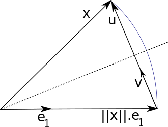
- It is obvious that: $\bs{\hat u}$ must be in the direction of $\bs u = \bs x - \Vert \bs x \Vert_2 \hat{\bs e}_1$.
QR decomposition using Householder
We show how to use Householder transformation to perform QR decomposition of the $A$ in previous example.
- The first step, zero out the lower triangle of the first column by a Householder transformation
def householder(x0, e=0) :
    n = len(x0)
    e1 = np.zeros(n-e)
    x = x0[e:]
    e1[0] = np.linalg.norm(x, 2)
    u = x - e1
    v = np.matrix(u/np.linalg.norm(u, 2))
    hs = np.eye(n-e) - 2*v.T*v
    h = np.eye(n)
    h[e:,e:] = hs
    return h

x, u, e1, Q, R = sp.symbols("x, u, e_1, Q, R")
xn = sp.symbols("\Vert{x}\Vert_2")
b = a[:, 0]
c = np.zeros(len(b))
c[0] = np.linalg.norm(b, 2)

fmt.displayMath(fmt.joinMath('=', A, sp.Matrix(np.round(a))), fmt.joinMath('=', x, sp.Matrix(a[:,0])),
                fmt.joinMath('=', xn, np.round(np.linalg.norm(b, 2), 3)),
                fmt.joinMath('=', e1, sp.Matrix([1, 0, 0, 0])),
                fmt.joinMath('=', u, sp.Matrix(a[:,0]-c).evalf(3)), pre="\\tiny ")

fmt.displayMath("\;")

h1 = householder(a[:, 0], 0)
H1 = sp.MatrixSymbol('H_1', 4, 4)
a1 = h1.dot(a)
fmt.displayMath(fmt.joinMath('=', H1, sp.Matrix(np.round(h1, 3))),
                fmt.joinMath('=', H1*A, sp.Matrix(np.round(a1, 3))), pre="\\tiny ")
continue to zero out the lower triangle
h2 = householder(a1[:, 1], 1)
H2 = sp.MatrixSymbol('H_2', 4, 4)
a2 = h2.dot(a1)
fmt.displayMath(fmt.joinMath('=', H2, sp.Matrix(np.round(h2, 3))),
                fmt.joinMath('=', H2*H1*A, sp.Matrix(np.round(a2, 3))), pre="\\tiny ")
fmt.displayMath("\;")

h3 = householder(a2[:, 2], 2)
H3 = sp.MatrixSymbol('H_3', 4, 4)
a3 = h3.dot(a2)
fmt.displayMath(fmt.joinMath('=', H3, sp.Matrix(np.round(h3, 3))),
                fmt.joinMath('=', H3*H2*H1*A, sp.Matrix(np.round(a3, 3))), pre="\\tiny ")
the final results are therefore $Q = (H_3H_2H_1)^T, R = Q^T A$:
q = (h3.dot(h2).dot(h1)).T
r = q.T.dot(a)
np.round(q.dot(r), 4)

fmt.displayMath(fmt.joinMath('=', Q, sp.Matrix(np.round(q, 3))), fmt.joinMath('=', R, sp.Matrix(np.round(r, 3))), pre="\\tiny ")
QR decomposition for least square
$$ \min_{\bs {\beta}} \Vert X \bs{\beta - y} \Vert_2$$
given the QR decomposition of $X = QR$:
$$ \min_{\bs {\beta}} \Vert X \bs{\beta - y} \Vert_2 = \min_{\bs {\beta}} \Vert Q^T X \bs \beta - Q^T \bs y \Vert_2 = \min_{\bs {\beta}} \Vert R \bs \beta - \bs y'\Vert_2$$
note that $R$ is right triangular, the vector whose norm is to be minimized looks like:
$$\scriptsize \begin{pmatrix} r_{11} & r_{12} & \cdots & r_{1n} \\ 0 & r_{22} & \cdots & r_{2n} \\ \vdots & \ddots & \ddots & \vdots \\ 0 & \cdots\ & 0 & r_{nn} \\ \hline 0 & 0 & \cdots & 0 \\ \vdots & \vdots & \ddots & \vdots \\ 0 & 0 & \cdots & 0 \end{pmatrix} \begin{pmatrix} \beta_1 \\ \beta_2 \\ \vdots \\ \beta_n \end{pmatrix} - \begin{pmatrix} y'_1 \\ y'_2 \\ \vdots \\ y'_n \\ \hline y'_{n+1} \\ \vdots \\ y'_m \end{pmatrix} $$
therefore, the solution is the $\bs \beta$ that zero out the first $n$ elements of the vector.
Top 10 numerical algorithm in the 20th century
By SIAM:
- 1946, Monte Carlo
- 1947, Simplex method for linear programming
- 1950, Subspace iteration for solving $A\bs x = \bs y$
- 1951, LU decomposition
- 1957, Fortran optimized compiler
- 1959-1961, QR decomposition/QR algorithm
- 1963, quicksort
- 1965, fast fourier transform
- 1977, integer relation detection algorithm
- 1987, fast multipole algorithm
Why single out the 20th century?

Principal Component Analysis
Mahatma Gandhi: action expresses priorities. $\renewcommand{bt}[1]{\tilde{\bs #1}}$
Principal component (PC)
Suppose $\tilde {\bs r}$ is a random vector, with expectation $\bar{\bs r} = \mathbb{E}[\tilde{\bs r}]$ and covariance matrix $ V = \mathbb{E}[(\bt r - \bar{\bs r})(\bt r - \bar{\bs r})^T] $
- e.g.: returns of a set of equity names
PC is defined to be the direction $\hat{\bs u}$ onto which the projection $\tilde {\bs r}^T \hat{\bs u}$ has the maximum variance,
- $\hat{\bs u}$ is a unit vector, i.e., $\Vert \hat{\bs u} \Vert_2 = \sqrt{\hat{\bs u}^T\hat{\bs u}} = 1$
es = np.random.normal(size=[3, 300])
x = (1.5*es[0,:] + .25*es[1,:])*.3 + 1
y = es[0,:]*.4 + es[2,:]*.2

cov = np.cov([x, y])
ev, evec = np.linalg.eig(cov)

ux = mean(x)
uy = mean(y)

figure(figsize=[6, 4])
plot(x, y, '.')
xlim(-2, 4)
ylim(-2, 2);
xlabel('x')
ylabel('y');

arrow(ux, uy, -3*sqrt(ev[1])*evec[0, 1], -3*sqrt(ev[1])*evec[1, 1], width=.01, color='r')
arrow(ux, uy, 3*sqrt(ev[0])*evec[0, 0], 3*sqrt(ev[0])*evec[1, 0], width=.01, color='r');
title('Principal Components of 2-D Data');

Link to eigenvectors
The projection $\hat{\bs u}^T \bt r$ is a random scalar:
- the variance of the projection is $\text{var}[\hat{\bs u}^T \bt r] = \hat{\bs u}^T V \hat{\bs u}$.
- the first eigen vector $\bs v_1$ of $V$ is therefore the principal component
If we limit ourselves to all $\bs u$ that is perpendicular to $\bs v_1$, then:
- the second eigen vector $\bs v_2$ of $V$ is the principal component amongst all $\bs u$ with $\bs v_1^T \bs u = 0$
- this process can continue for all the eigen vectors
Variance explained
The total variance of the random vector $\tilde {\bs r}$ is sum of variance of all its $n$ elements, which equals:
- trace of $V$
- sum of all eigen values of $V$
The portion of variance explained by the first $k$ eigenvectors is $\frac{\sum_i^k \lambda_i}{\sum_i^n \lambda_i}$.
Application in interest rates
CMT rates are constant maturity treasury bond yield that are published daily by U. S. Treasury.
cmt_rates = pd.read_csv("data/cmt.csv", parse_dates=[0], index_col=[0])

cmt_rates.plot(legend=False, title='Historical CMT yield');

Covariance matrix
- Covariance matrix between CMT rates at different maturities
tenors = cmt_rates.columns.map(float)
cv = cmt_rates.cov()
fmt.displayDF(cv, "4g")
IR PCA components
The eigenvectors and percentage explained,
- the 1st principal component (PC) explains >95% of the variance
- the first 3 PCs can be interpreted as level, slope and curvature
- note that the sign of the PC is insignificant
xcv, vcv = np.linalg.eig(cv)
vcv = -vcv # flip the sign of eigen vectors for better illustratiaons

pct_v = np.cumsum(xcv)/sum(xcv)*100

import pandas as pd
pd.set_option('display.precision', 3)
fmt.displayDF(pd.DataFrame({'P/C':range(1, len(xcv)+1),
                            'Eigenvalues':xcv, 'Cumulative Var(%)': pct_v}).set_index(['P/C']).T, "2f")
flab = ['factor %d' % i for i in range(1, 4)]

fig = figure(figsize=[12, 4])
ax1 = fig.add_subplot(121)
plot(tenors, vcv[:, :3], '.-');
xlabel('Tenors(Y)')
legend(flab, loc='best')
title('First 3 principal components');

fs = cmt_rates.dot(vcv).iloc[:, :3]

ax2 = fig.add_subplot(122)
fs.plot(ax=ax2, title='Projections to the first 3 P/Cs')
legend(flab, loc='best');

Dimension reduction in MC
Given a generic $n$-dimensional SDE in vector form:
$$\renewcommand{Sigma}{\mathcal{S}} d \bs x = \bs u dt + A \Sigma d \bs w, \;\;\; d\bs w d\bs w^T = C dt$$
- $\Sigma$ is a diagonal matrix of $\sigma_i$
- $C$ is the correlation matrix of $\Sigma d \bs w$, its covariance matrix $V = \Sigma C \Sigma$.
Recall Cholesky decomposition $V = LL^T$: $\Sigma \delta \bs w = L \bt z \sqrt{\delta t}$:
$$ \small \mathbb E [\Sigma\delta \bs w (\Sigma\delta \bs w)^T] = \mathbb E[(L \delta t \bt z \sqrt{\delta t}) (L \delta t \bt z \sqrt{\delta t})^T ] = L \mathbb E[\delta t \bt z\delta t \bt z^T] L^T \delta t = V \delta t $$
- $\bt z$ is independent standard normal random vector.
- we can reduce $\bt z$ dimension by finding a rectangular $\dot L$ so that $V \approx \dot L {\dot L}^T$
Dimension reduction with PCA
Use the PCA of the covariance matrix: $$ \scriptsize V = R_V \Lambda_V R_V^T \approx \dot R_V \dot \Lambda_V \dot R_V^T = \dot R_V \dot H_V \dot H_V^T \dot R_V^T = (\overbrace{\dot R_V \dot H_V}^{L_V})(\dot R_V\dot H_V )^T \\$$ Or PCA on the correlation matrix: $$ \scriptsize V = \Sigma C \Sigma = \Sigma (R_C \Lambda_C R_C^T) \Sigma \approx \Sigma \dot R_C \dot \Lambda_C \dot R_C^T \Sigma = \Sigma \dot R_C \dot H_C \dot H_C^T \dot R_C^T \Sigma^T = (\overbrace{\Sigma \dot R_C \dot H_C}^{L_C})(\Sigma \dot R_C\dot H_C )^T $$
- $\Lambda = H H^T$, both $\Lambda$ and $H$ are diagonal matrix with positive elements
- The dotted version only retains the first $k$ eigen values
- $\dot R$ and $L_V, L_C$ are $n \times k$ matrices; $\dot \Lambda$ are $k \times k$ matrices.
Simulation can then be driven by $\Sigma \delta \bs w = L \dot{\bt z} \sqrt{\delta t}$:
- Either $L_V = \dot R_V \dot H_V$ or $L_C = \Sigma \dot R_C \dot H_C$ works
- $\dot{\bt z}$ is of length $k$ only
PCA is scale variant
Given the EVDs on covariance and correlation matrices:
$$R_V \Lambda_V R_V^T = V = \Sigma C \Sigma = \Sigma R_C \Lambda_C R_C^T \Sigma$$
Are they equivalent?
- $\Sigma R_C \Lambda_C R_C^T \Sigma = (\Sigma R_C) \Lambda_C (\Sigma R_C)^T$
- implies $\Lambda_C = \Lambda_V$ and $R_V = \Sigma R_C$
- $\Sigma R_C \Lambda_C R_C^T \Sigma = R_C (\Sigma \Lambda_C \Sigma) R_C^T$
- implies $ \Lambda_V = \Sigma \Lambda_C \Sigma $ and $R_C = R_V$
However, neither is true because:
- $\Sigma R_C$ is not orthogonal: $(\Sigma R_C)(\Sigma R_C)^T = \Sigma R_C R_C^T \Sigma = \Sigma\Sigma \ne I$
- $V = \Sigma C \Sigma$, $V$ and $C$ are not similar
- $\Sigma R_C \ne R_C \Sigma$, even when $\Sigma$ is diagonal.
There is no simple relationship btw these two EVDs.
- despite $C$ and $V$ are covariance matrix of $\bt r$ and $\Sigma^{-1} \bt r$ respectively
Orthogonality depends on scale
The PCs are no longer orthogonal after stretching horizontally.
figure(figsize=[13, 4])
subplot(1, 2, 1)

plot(x, y, '.')
xlim(-2, 4)
ylim(-2, 2);
xlabel('x')
ylabel('y');

arrow(ux, uy, -3*sqrt(ev[1])*evec[0, 1], -3*sqrt(ev[1])*evec[1, 1], width=.01, color='r')
arrow(ux, uy, 3*sqrt(ev[0])*evec[0, 0], 3*sqrt(ev[0])*evec[1, 0], width=.01, color='r');
title('Unscaled PCs');

subplot(1, 2, 2)

scale = 1.5
plot(x*scale, y, '.')
xlim(-2, 4)
ylim(-2, 2);
xlabel('x')
ylabel('y');

arrow(ux*scale, uy, -3*sqrt(ev[1])*evec[0, 1]*scale, -3*sqrt(ev[1])*evec[1, 1], width=.01, color='r')
arrow(ux*scale, uy, 3*sqrt(ev[0])*evec[0, 0]*scale, 3*sqrt(ev[0])*evec[1, 0], width=.01, color='r');
title('Scaled');

Before applying PCA
PCA is a powerful technique, however, beware of its limitations:
- PCA factors are not real market risk factors
- It does not lead to tradable hedging strategies
- PCA is not scale (or unit) invariant
- it requires all the dimensions to have the same natural unit
- mixing factors of different magnitude can lead to trouble: eg, mixing interest rates with equities
- PCA results are different when applied to co-variance matrix and correlation matrix
PCA is usually applied to different data points of the same type
- different tenors/strikes of interest rates, volatility etc.
- price movements of the same sector/asset class
PCA vs. least square
The PCA analysis has some similarity to the least square problem, both of them can be viewed as minimizing the L2 norm of residual errors.
xs = np.array([x, np.ones(len(x))]).T
beta = np.linalg.inv(xs.T.dot(xs)).dot(xs.T).dot(y)

s_x, s_y = sp.symbols('x, y')
br = np.round(beta, 4)

figure(figsize=[13, 4])
subplot(1, 2, 1)
plot(x, y, '.')
xlim(-2, 4)
ylim(-2, 2);
xlabel('x')
ylabel('y');

dx = 4*sqrt(ev[0])*evec[0, 0]
dy = 4*sqrt(ev[0])*evec[1, 0]

arrow(ux-dx, uy-dy, 2*dx, 2*dy, width=.01, color='k');

ex = 3*sqrt(ev[1])*evec[0, 1]
ey = 3*sqrt(ev[1])*evec[1, 1]
plot([ux, ux+ex], [uy, uy+ey], 'r-o', lw=3)
legend(['data', 'residual error'], loc='best')

title('PCA');

subplot(1, 2, 2)
plot(x, y, '.')
xlim(-2, 4)
ylim(-2, 2);
xlabel('x')
ylabel('y');
arrow(-1, -1*beta[0]+beta[1], 4, 4*beta[0], width=.01, color='k');
y0 = (ux+ex)*beta[0] + beta[1]
plot([ux+ex, ux+ex], [y0, uy+ey], 'r-o', lw=3)
legend(['data', 'residual error'], loc='best')
title('Least Square');

PCA or regression?
The main differences between PCA and least square (regression):
| PCA | Least Square/Regression | |
|---|---|---|
| Scale Invariant | No | Yes |
| Symmetry in Dimension | Yes | No |
To choose between the two:
- Use least square/regression when there are clear explanatory variables and causality
- Use PCA when there is a set of related variables but no clear causality
- PCA requires a natural unit for all dimensions
What variable to apply PCA
It is important to choose the right variable to apply PCA. The main considerations are:
Values or changes
- Equity prices or returns?
- IR levels or changes?
- Key consideration: stationarity and mean reversion, horizon of your model prediction
Spot or forward
- Forward is usually a better choice than spot
Since the PCA is commonly applied to a correlation/covariance matrix, it is equivalent to ask what variables' correlation/covariance matrix we should model.
Spurious correlation - equity price
Spurious correlation: variables can appear to be significantly correlated, but it is just an illusion:
f3 = pd.read_csv('data/f3.csv', parse_dates=[0]).set_index('Date').sort_index()
r = np.log(f3).diff()

fmt.displayDFs(f3.corr(), r.corr(), headers=['Price Correlation', 'Return Correlation'], fmt="4g")
Spurious correlation - spot rates
The correlation between 9Y and 10Y spot rates and forward rates:
es = np.random.normal(size=[2, 500])
r0 = es[0,:]*.015 + .05
f1 = es[1,:]*.015 + .05

r1 = -np.log(np.exp(-9*r0-f1))/10


rc = np.corrcoef(np.array([r0, r1]))[0, 1]
fc = np.corrcoef(np.array([r0, f1]))[0, 1]

figure(figsize=[12, 4])
subplot(1, 2, 1)
plot(r0, r1, '.')
xlabel('9Y rate')
ylabel('10Y spot')
title('Corr(9Y Spot, 10Y Spot) = %.4f'% rc)

subplot(1, 2, 2)
plot(r0, f1, '.')
xlabel('9Y rate')
ylabel('9-10Y forward')
title('Corr(9Y Spot, 9-10Y Forward) = %.4f'% fc);

$$\begin{eqnarray} \exp(-10 r_{10}) &=& \exp(-9 r_9)\exp(-(10-9) f(9, 10) ) \\ r_{10} &=& 0.9r_9 + 0.1f(9, 10) \end{eqnarray}$$
- the $f(9, 10)$ is the 9Y to 10Y forward rate.
- of course $r_{10} = f(0, 10)$
Correlated by construction
$$ r_{10} = 0.9r_9 + 0.1f(9, 10) $$
- The high correlation between spot rates to similar tenors are by construction
- PCA analysis can be misleading in percentage of variance explained
- the variance of spot rates of short tenors are counted multiple times
- May not be a problem if we have unlimited precision, but we usually only keep the first few eigen vectors in PCA
- it's usually better to model the correlation/covariance matrix of forward rates
Singular Value Decomposition
rotate, stretch and rotate, then you get back to square one, that's pretty much the life in a bank.
Definition
For any real matrix $M$, $\sigma \geq 0$ is a singular value if there exists two $\bf\mbox{unit-length}$ ectors $\bs {u, v}$ such that:
- $M \bs v = \sigma \bs u$
- $\bs u^T M = \sigma \bs v^T$
$\bs {u, v}$ are called left and right singular vector of $M$.
- unlike eigenvalues, singular values are always non-negative.
By convention,
- we represent singular vectors as unit L-2 vectors, i.e., $\bs u^T\bs u = \bs v^T \bs v = 1$,
- we name the singular values in descending order as $\sigma_1, \sigma_2, ..., \sigma_n$, and refer corresponding singular vector pairs as $ (\bs u_1, \bs v_1), (\bs u_2, \bs v_2), ..., (\bs u_n, \bs v_n) $.
Singular vectors and maximization
Consider $\bs u^T M \bs v$ for real matrix $M$:
- $\bs {u_1, v_1}$ maximize $\bs u^T M \bs v$ amongst all unit $\bs {u, v}$ vectors.
Apply the Lagrange multiplier, with constraints $\bs u^T \bs u = \bs v^T \bs v = 1$:
$$\small \begin{array} \\l &= \bs u^T M \bs v - \lambda_1 (\bs u^T \bs u - 1) - \lambda_2 (\bs v^T \bs v - 1) \\ \frac{\partial l}{\partial{\bs u^T}} &= M \bs v - 2 \lambda_1 \bs u = \bs 0 \iff \bs u^T M \bs v - 2 \lambda_1 = \bs 0\\ \frac{\partial l}{\partial{\bs v}} &= \bs u^T M - 2\lambda_2 \bs v^T = \bs 0^T \iff \bs u^T M \bs v- 2\lambda_2 = \bs 0 \end{array}$$
Therefore, $$ 2\lambda_1 = \small \bs u^T M \bs v = 2\lambda_2 $$ $$M \bs v = \sigma \bs u \;,\; M^T\bs u = \sigma \bs v $$
Orthogonality of Singular Vectors
Given $\bs{u_1, v_1}$ are the first singular vectors of $M$:
$$\bs x^T \bs v_1 = 0 \iff (M \bs x)^T \bs u_1 = 0 \iff \bs u_1^T M \bs x = 0 $$
because:
$$ (M \bs x)^T \bs u_1 = \bs x^T M^T \bs u_1 = \bs x^T \sigma_1 \bs v_1 = 0 $$
Therefore, if we only consider those $\bs u^T M^T \bs u_1 = 0$ ($M$-orthogonal), the corresponding $\bs v$ must be orthogonal to $\bs v_1$ :
- $\bs {u_2, v_2}$ maximizes $\bs u^T M \bs v$ among those $(\bs u, \bs v)$ orthogonal to $\bs u_1, \bs v_1$
- this process can repeat for all singular vectors (assuming singular values are distinct)
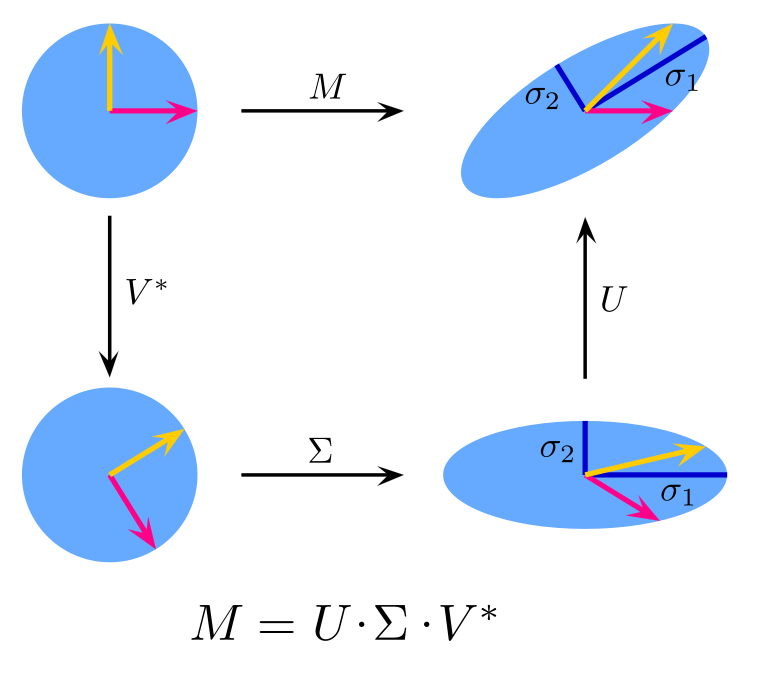
Singular value decomposition
We can write all singular vectors and singular values in matrix format, which is the singular value decomposition (SVD):
$$ U^T M V = \Sigma \iff M = U \Sigma V^T $$
| $M$ | $U$ | $\Sigma$ | $V$ | |
|---|---|---|---|---|
| Name | Original Matrix | Left singular vector | Singular value | Right singular vector |
| Type | Real | Orthogonal, real | Diagonal, positive | Orthogonal, real |
| Size | $m \times n$ | $m\times m$ | $m\times n$ | $n \times n$ |
- For matrix $M$, there can only be $\min(m, n)$ singular values at most
- The left/right singular vectors form a basis for the vector space of $\bs {u}$ and $\bs v$ respectively
Link between SVD and EVD
$$ M = U \Sigma V^T $$
SVD and eigenvalue decomposition (EVD) are closely related to each other:
- SVD reduces to EVD if $M$ is symmetric positive definite
- $MM^T = U \Sigma V^T V \Sigma^T U^T = U \Sigma \Sigma^T U^T$:
- the column vectors of $U$ are the eigen vectors of $MM^T$
- $M^TM = V\Sigma^TU^TU\Sigma V^T = V \Sigma\Sigma^T V^T$:
- the column vectors of $V$ are the eigen vectors of $M^TM$
- The singular values are the positive square roots of eigen values of $MM^T$ or $M^TM$
SVD of pseudo inverse
Given the SVD decomposition $X = U\Sigma V^T$, the SVD of $X$'s pseudo inverse is:
$$X^+ = (X^TX)^{-1}X^T = V \Sigma^+ U^T$$
where $\Sigma^+$ is the pseudo inverse of $\Sigma$, whose diagonal elements are the reciprocals of those in $\Sigma$.
Proof: the last equation is obviously true, and every step is reversible:
$$\begin{array}&(X^TX)^{-1}X^T &= V\Sigma^+ U^T \\ (V \Sigma^T \Sigma V^T)^{-1} V\Sigma^TU^T &= V\Sigma^+ U^T \\ (V \Sigma^T \Sigma V^T)^{-1} V\Sigma^T\Sigma &= V \Sigma^+\Sigma \\ (V \Sigma^T \Sigma V^T)^{-1} V\Sigma^T\Sigma &= V \\ (V \Sigma^T \Sigma V^T)^{-1} (V\Sigma^T\Sigma V^T) &= I \end{array}$$
SVD is another way to solve the least square problem.
L2 norm and condition number
Consider a real matrix $A$, its L2 norm is defined as the maximum of $\frac{\Vert A \bs x \Vert_2}{\Vert \bs x \Vert_2}$:
$$ \Vert A \Vert_2^2 = \max_{\bs x} \frac{\Vert A \bs x \Vert_2^2}{\Vert \bs x \Vert_2^2} = \max_{\bs x} \frac{\bs x^T A^T A \bs x}{\bs x^T \bs x} = \max_{\hat{\bs x}} \hat{\bs x}^T A^T A \hat{\bs x} = \sigma_1(A)^2$$
where $\hat{\bs x} = \frac{\bs x}{\Vert \bs x \Vert_2}$ is a unit vector, and $\sigma_1(A)$ is the largest singular value of $A$.
For a generic non-square matrix $A$:
- the L-2 norm of a matrix is its largest singular value: $\Vert A \Vert_2 = \sigma_1(A)$
- the L-2 norm of the pseudo inverse $A^+$: $\Vert A^+ \Vert_2 = \frac{1}{\sigma_n(A)}$
- $\sigma_n(A)$ is the smallest singular value of $A$.
- the L-2 condition number of a matrix $A$ is therefore: $k(A) = \Vert A \Vert_2 \Vert A^+ \Vert_2 = \frac{\sigma_1(A)}{\sigma_n(A)}$
SVD and condition number
SVD offers clear intuitions in understanding the L-2 condition number of a Matrix $A$.
For a linear system $\bs y = A \bs x$, consider a perturbation $\delta \bs x$ to the input $\bs x$:
- if $\delta \bs x$ is stretched by a larger factor than $\bs x$, then the relative error grows.
- the worst case occurs when $\bs x$ is stretched by $\sigma_n(A)$, while $\delta \bs x$ is stretched by $\sigma_1(A)$
- the relative error grows by a factor of $\frac{\sigma_1(A)}{\sigma_n(A)}$.
- Orthogonal matrix represents a pure rotation
- all singular values are 1, no stretches, thus the relative error does not grow
Spot the trouble
When working with near singular matrix, SVD can identify ill-conditioned area:
- real world covariance and correlation matrix are often near singular
- numerical instability arises when inputs are very close to signular vectors with small singular values
- e.g, when return forecast is in the same direction as the last singular vector ...
Rank deficiency and reduction
Singular matrix are those that are not fully ranked
- Square matrix: non-invertible, its determinant is 0
- In practice, matrices are rarely exactly singular due to numerical errors
SVD can detect near singular matrices
- near singular matrix has very small singular values
SVD can find low rank approximations to a full rank matrix
- by zeroing out small singular values
Condition number for EVD
What is the change in $\lambda_i$ if we perturb the symmetric matrix $A$?
$$ A \bs v_i = \lambda_i \bs v_i$$
Apply the perturbation analysis: $\delta A = \dot{A} \epsilon, \delta \lambda_i = \dot{\lambda_i} \epsilon, \delta \bs v_i = \dot{\bs v_i} \epsilon$, the first order terms of $\epsilon$:
$$\begin{array} \\ (A + \dot{A}\epsilon )(\bs v_i + \dot{\bs v_i}\epsilon) &= (\lambda_i + \dot{\lambda_i}\epsilon) (\bs v_i + \dot{\bs v_i} \epsilon) \\ \dot{A}\bs v_i + A \dot{\bs v_i} &= \lambda_i \dot{\bs v_i} + \dot{\lambda_i}\bs v_i \\ \bs v_i^T\dot{A}\bs v_i + \bs v_i^T A \dot{\bs v_i} &= \bs v_i^T \lambda_i \dot{\bs v_i} + \bs v_i^T \dot{\lambda_i}\bs v_i \\ \bs v_i^T\dot{A}\bs v_i &= \dot{\lambda_i} \end{array}$$
Therefore: $$\begin{array} \\ \frac{ | \delta \lambda_i |}{| \lambda_i |} &= \frac{\Vert \bs v_i^T\delta A \bs v_i\Vert_2}{|\lambda_i|} \le \frac{\Vert \delta A \Vert_2}{|\lambda_i|} = \frac{\Vert A\Vert_2}{|\lambda_i|} \frac{\Vert \delta A \Vert_2}{\Vert A \Vert_2} = \left\vert \frac{\lambda_1}{\lambda_i}\right\vert \frac{\Vert \delta A \Vert_2}{\Vert A \Vert_2} \end{array}$$
- The eigenvalue's conditional number for a symmetric matrix $A$ is therefore the ratio from the largest eigen value: $k(A) = \left\vert \frac{\lambda_1}{\lambda_i} \right\vert$.
- The smaller eigenvalues are less accurate, we should ignore them.
Decomposition summary
For real matrix $A$:
| Decomposition | Applicability | Formula | Results | Key applications |
|---|---|---|---|---|
| LU | square, full rank | $A = LU$ | lower, upper triangular | matrix inversion |
| Cholesky | symmetric positive definite | $A = LL^T$ | lower triangular | simulate correlated factors |
| QR | any | $A = Q R$ | orthogonal, upper triangular | solve eigen values, least square |
| EVD | symmetric | $A = R\Lambda R^T$ | orthogonal, real diagonal | PCA |
| SVD | any | $A = U\Sigma V^T$ | orthogonal, positive diagonal, orthogonal | error analysis, rank reduction |
Assignment
Required reading:
- Bindel and Goodman: Chapter 4
Recommended reading:
- Andersen and Piterbarg: 4.1
Homework: